Fisher's exact test
Fisher’s exact test computes an exact p-value for a 2x2 contingency table. Unlike the chi-square test, it does not rely on a large-sample approximation: it conditions on the table’s fixed marginal totals and computes probabilities directly from the hypergeometric distribution, which makes it reliable even with very small samples.
Why an exact test?
Consider a 2x2 table with cells \(a, b, c, d\), where the rows sum to \(a+b\) and \(c+d\), the columns sum to \(a+c\) and \(b+d\), and the grand total is \(n\):
| Outcome 1 | Outcome 2 | Total | |
|---|---|---|---|
| Group 1 | \(a\) | \(b\) | \(a+b\) |
| Group 2 | \(c\) | \(d\) | \(c+d\) |
| Total | \(a+c\) | \(b+d\) | \(n\) |
If we condition on all four marginal totals being fixed, only cell \(a\) is free to vary: once \(a\) is known, \(b\), \(c\) and \(d\) are all determined by subtraction from the margins. Under \(H_0\) of independence, \(a\) then follows a hypergeometric distribution:
\[P(a) = \frac{\binom{a+b}{a}\binom{c+d}{c}}{\binom{n}{a+c}}\]
This is exactly the probability of drawing \(a\) “successes” when sampling \(a+c\) items without replacement from a population of \(n\) items containing \(a+b\) successes in total. Because this probability is computed directly, with no reliance on a large-sample approximation, the resulting p-value is exact rather than asymptotic. The exact p-value sums the hypergeometric probabilities of all tables at least as extreme as the observed one, that is, all tables with the same fixed margins that are as supportive of \(H_1\) as the observed table, or more so.
Hypotheses
| Test | \(H_0\) | \(H_1\) |
|---|---|---|
| Two-sided | the variables are independent (OR = 1) | the variables are associated (OR \(\neq\) 1) |
| One-sided (less) | OR \(\geq\) 1 | OR \(<\) 1 |
| One-sided (greater) | OR \(\leq\) 1 | OR \(>\) 1 |
\(H_0\) states that the two categorical variables are independent, which is equivalent to saying the odds ratio equals 1. \(H_1\) for the two-sided test states that the variables are associated, that is, the odds ratio differs from 1. The one-sided versions test a specific direction of association, chosen before looking at the data.
The odds ratio
The odds ratio measures the strength and direction of the association:
\[\text{OR} = \frac{ad}{bc}\]
An odds ratio of 1 means no association: the odds of the outcome are the same in both groups. An odds ratio greater than 1 means the outcome is more likely in the first row or group, while an odds ratio less than 1 means it is less likely.
R’s fisher.test() does not report this simple cross-product. Instead, it reports a bias-corrected estimate known as the conditional maximum likelihood estimate (conditional MLE) of the odds ratio. This value is close to, but not identical to, \(ad/bc\). Both are legitimate estimates of the same underlying association; the simple cross-product is easier to compute by hand, while the conditional MLE is the one that matches the confidence interval R reports alongside the p-value.
Examples
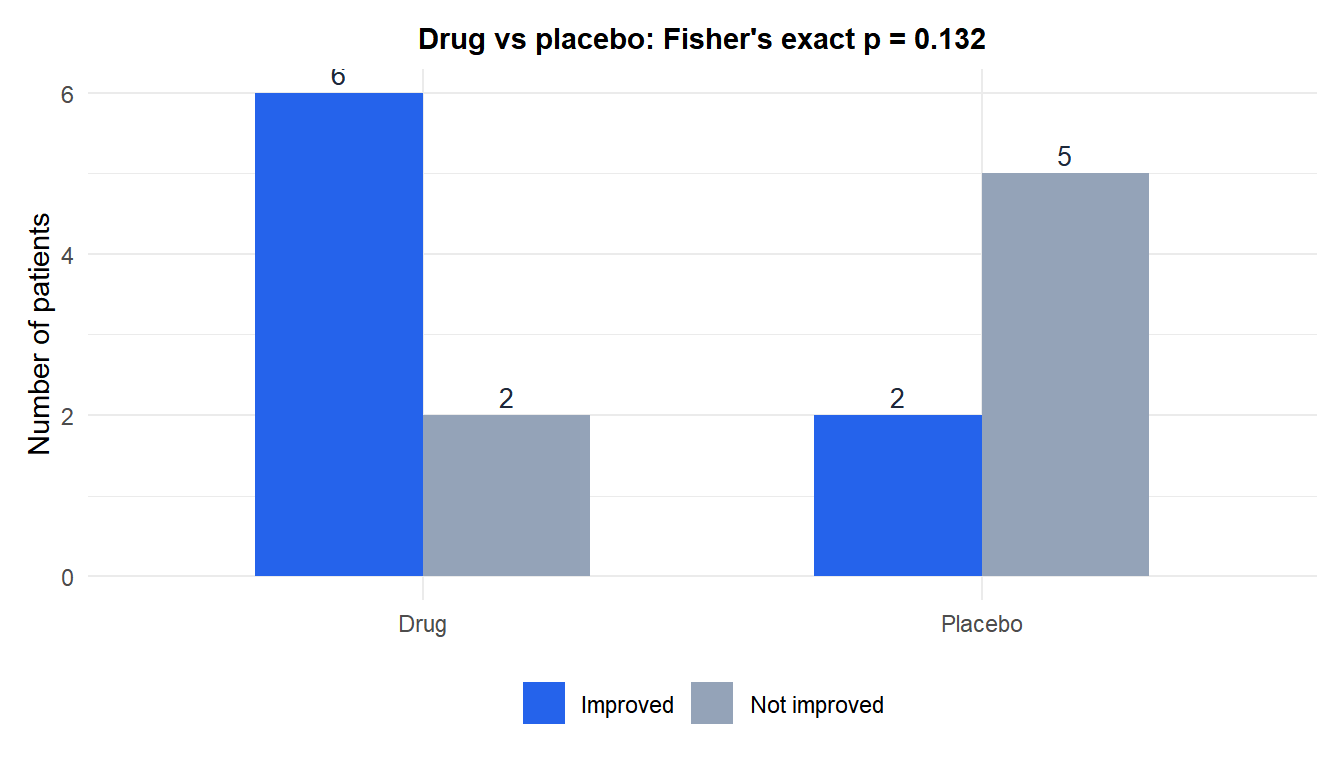
Example 1: small clinical trial, new drug vs placebo (two-sided)
A small trial has too few patients for the chi-square approximation to be trusted:
| Improved | Not improved | Total | |
|---|---|---|---|
| Drug | 6 | 2 | 8 |
| Placebo | 2 | 5 | 7 |
| Total | 8 | 7 | 15 |
Expected counts here are as low as 3.27 in one cell, well under the usual rule of thumb of 5, so chi-square would not be reliable.
Cross-product odds ratio: \(OR = (6 \times 5)/(2 \times 2) = 30/4 = 7.5\).
Fisher’s exact test (R’s conditional MLE estimate: OR = 6.40) gives a two-sided p-value of 0.132.
Decision: fail to reject \(H_0\) at \(\alpha=0.05\). Despite the descriptively large odds ratio, the sample is too small to call the association statistically significant.

Example 2: vaccine efficacy trial (one-sided)
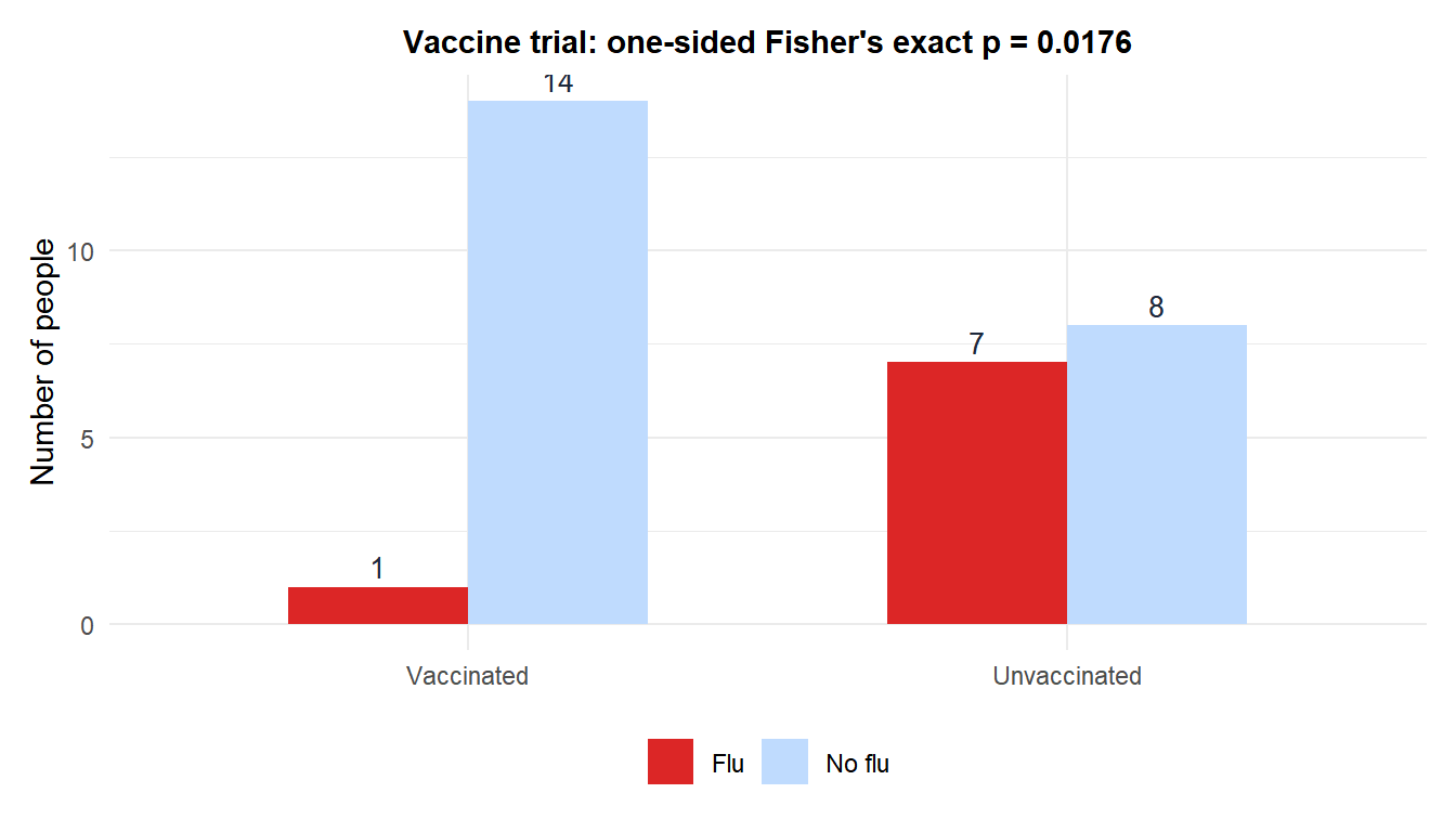
15 people are vaccinated, 15 are not; the outcome is whether they caught the flu that season:
| Flu | No flu | Total | |
|---|---|---|---|
| Vaccinated | 1 | 14 | 15 |
| Unvaccinated | 7 | 8 | 15 |
| Total | 8 | 22 | 30 |
Hypotheses: \(H_0\): vaccination does not reduce flu risk (OR \(\geq\) 1) vs \(H_1\): vaccination reduces flu risk (OR \(<\) 1), a one-sided test since the researchers have a specific directional hypothesis.
Cross-product odds ratio: \(OR = (1 \times 8)/(14 \times 7) = 8/98 \approx 0.082\).
One-sided (“less”) p-value: 0.0176. Two-sided p-value (for comparison): 0.0352.
Decision (one-sided): reject \(H_0\) at \(\alpha=0.05\). There is significant evidence that vaccination reduces flu risk in this sample.
Assumptions
Fisher’s exact test requires:
- Fixed margins: both the row and column totals are treated as fixed. This is the classical, conditional framing of the test; treating both margins as fixed is itself a long-standing point of statistical debate, but it remains the standard practical approach.
- Independence: observations are independent of one another.
- No sample size restriction: unlike chi-square, there is no requirement on expected cell counts. That is the whole point of the test: it works even when chi-square’s rule of thumb (expected counts \(\geq 5\)) fails.
Fisher’s exact test is normally used only for 2x2 tables. Larger tables need the generalized Freeman-Halton extension, which is computationally intensive but available via fisher.test() in R, which also handles \(r \times c\) tables by simulation for large tables (simulate.p.value = TRUE).
⚠️ Fisher's exact test is not always more powerful, and can be conservative
A common misconception: “exact” does not mean “more powerful”. Because the test statistic (the count in one cell) is discrete, the achievable p-values form a coarse, discrete set, so the test can be conservative: its true rejection rate under \(H_0\) can be noticeably below the nominal \(\alpha\), especially with small, unbalanced tables. This is a real tradeoff against the chi-square approximation, which is anti-conservative in the same small-sample regime rather than the reverse.
In practice: use chi-square when expected counts are all \(\geq 5\), use Fisher’s exact test when they are not, and do not expect Fisher’s exact test to automatically detect a real effect just because it computes an “exact” answer.
Running the test in R
Both 2x2 examples above, plus a one-sided variant and a larger table handled by simulation, all through the same fisher.test() function:
# Example 1: clinical trial
tab1 <- matrix(c(6, 2, 2, 5), nrow = 2, byrow = TRUE)
fisher.test(tab1)                          # two-sided by default

# Example 2: vaccine trial (one-sided)
tab2 <- matrix(c(1, 14, 7, 8), nrow = 2, byrow = TRUE)
fisher.test(tab2, alternative = "less")    # one-sided
fisher.test(tab2)                          # two-sided, for comparison

# Larger tables (Freeman-Halton extension via simulation)
fisher.test(table_rxc, simulate.p.value = TRUE, B = 10000)
The output includes the p-value, the conditional MLE estimate of the odds ratio, and a confidence interval for the odds ratio. The alternative argument controls whether the test is two-sided (the default) or one-sided ("less" or "greater").
💡 Fisher's exact test vs chi-square: the decision rule
Use Fisher’s exact test for 2x2 tables when any expected cell count is below 5 (the chi-square approximation’s usual rule of thumb), or whenever the total sample size is small regardless of the exact counts. Use chi-square for larger, well-balanced tables: it is computationally lighter and its assumptions are already met. For tables larger than 2x2 with small counts, use fisher.test(..., simulate.p.value = TRUE) rather than the classical chi-square goodness-of-fit approximation.

