Jarque-Bera test
The Jarque-Bera test evaluates normality by checking two specific properties: skewness (symmetry) and excess kurtosis (tail weight). A normal distribution has skewness 0 and excess kurtosis 0. The test quantifies how far the sample departs from both, and combines them into a single chi-squared statistic.
Test statistic
The statistic combines the sample’s squared skewness and squared excess kurtosis into one number that should be small under normality:
\[JB = \frac{n}{6}\left(S^2 + \frac{(K-3)^2}{4}\right)\]
where \(n\) is the sample size, \(S\) is the sample skewness, and \(K\) is the sample excess kurtosis (so a normal distribution gives \(K-3 = 0\)). Under \(H_0\) (normality), \(JB\) follows a \(\chi^2\) distribution with 2 degrees of freedom for large \(n\).
The two terms are the two components of the test:
- \(S^2\): contribution from skewness. A skewed distribution increases this term.
- \((K-3)^2/4\): contribution from excess kurtosis. Heavy or light tails increase this term.
Hypotheses: \(H_0\): the data are normally distributed (\(S = 0\) and \(K = 3\)). \(H_1\): skewness and/or kurtosis deviate from normal values.
Decomposing non-normality
The JB test is unique among normality tests in that it tells you not just whether the data are non-normal, but in which way: via skewness, kurtosis, or both.
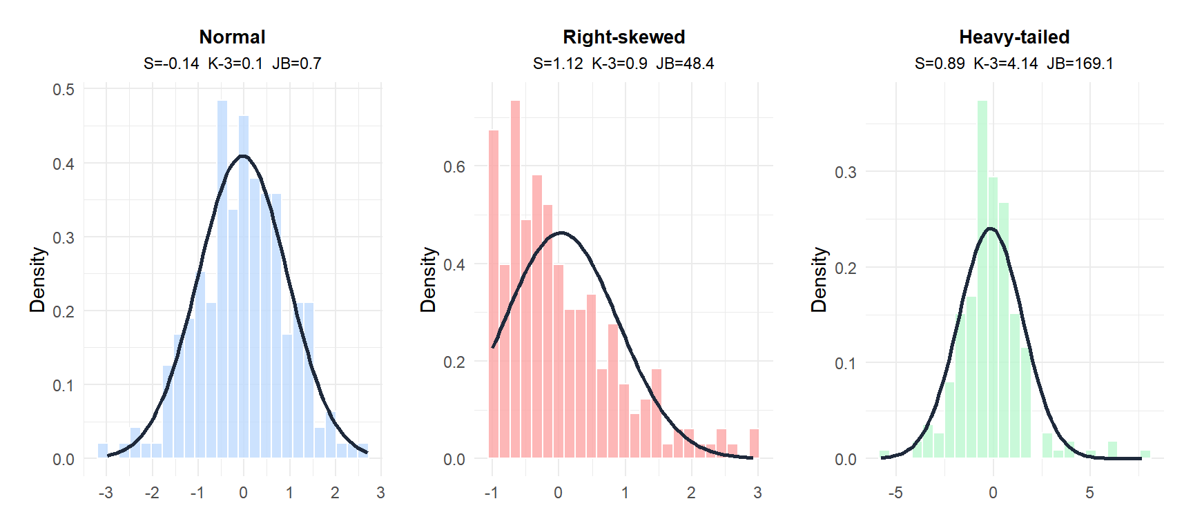
The normal data has \(S \approx 0\) and \(K-3 \approx 0\), giving a small JB. The skewed data has high \(|S|\), driven by asymmetry. The heavy-tailed data has high \(|K-3|\), driven by excess kurtosis, even if roughly symmetric.
Step-by-step example
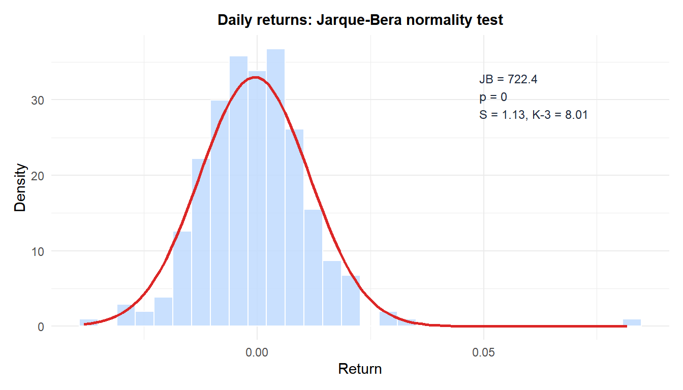
A financial analyst tests whether daily stock returns (\(n = 250\)) follow a normal distribution. The sample gives \(S = 0.61\) (mild right skew) and \(K = 4.82\) (slightly heavy tails, so \(K - 3 = 1.82\)).
Test statistic:
\[JB = \frac{250}{6}\left(0.61^2 + \frac{1.82^2}{4}\right) = 41.67 \times \left(0.372 + 0.828\right) = 41.67 \times 1.200 = 50.0\]
Critical value (\(\chi^2_{0.05, 2} = 5.991\)) and p-value (\(p \approx 0.000\)).
Decision: reject \(H_0\). The returns are significantly non-normal, with contributions from both skewness and excess kurtosis. This is typical of financial returns, which tend to be leptokurtic (fat tails) and slightly skewed.
Assumptions and limitations
The test’s main weakness is its reliance on an asymptotic approximation that only kicks in once the sample is reasonably large.
⚠️ The chi-squared approximation is unreliable for small samples
The \(\chi^2(2)\) p-value is only accurate for large samples. For \(n < 30\), the actual distribution of \(JB\) under \(H_0\) differs substantially from \(\chi^2(2)\), making p-values unreliable. For \(n < 100\), the approximation is still imperfect.
For small samples, use Shapiro-Wilk instead. The JB test is best suited for \(n \geq 100\), where it provides good power against both skewness and kurtosis departures.
⚠️ The test only captures skewness and kurtosis departures
The JB test is blind to departures from normality that do not manifest as changes in skewness or kurtosis. For example, a bimodal distribution with equal-sized symmetric modes can have \(S = 0\) and \(K \approx 3\), passing the JB test despite being clearly non-normal. Use a Q-Q plot alongside the formal test.
When to use JB vs Shapiro-Wilk
| Criterion | Jarque-Bera | Shapiro-Wilk |
|---|---|---|
| Best sample size | \(n \geq 100\) | \(3 \leq n \leq 5000\) |
| Power for small \(n\) | Low | High |
| Identifies departure type | Yes (skewness vs kurtosis) | No |
| Used in econometrics | Very common | Less common |
| R function | tseries::jarque.bera.test() |
shapiro.test() |
The JB test is standard in econometrics and finance, where large samples are common and interest in fat tails is high. For general statistics, Shapiro-Wilk is usually preferred.
Running the test in R
The JB test is available in the tseries and moments packages. Both give the same result:
library(tseries)
jarque.bera.test(x)

# Or manually:
library(moments)
n <- length(x)
S <- skewness(x)
K <- kurtosis(x)   # moments uses excess kurtosis by default
JB <- n/6 * (S^2 + (K - 3)^2 / 4)
p_val <- pchisq(JB, df = 2, lower.tail = FALSE)
💡 Practical workflow for normality in large samples
For \(n \geq 100\) where Shapiro-Wilk may be overpowered:
- Plot a histogram and Q-Q plot to visually assess the departure.
- Run the JB test to get a formal p-value.
- If rejected, check which component (\(S\) or \(K-3\)) drives the result: this guides the choice of remedy (transformation for skewness, robust methods or heavy-tailed distributions for kurtosis).
- Consider whether the downstream test is robust to the specific type of non-normality detected.

