McNemar's test
McNemar’s test compares two binary measurements taken on the same subjects, before/after, two raters, two diagnostic tests, unlike the chi-square test of independence, which assumes independent groups. It is the categorical-data analogue of the paired t-test: both exploit the pairing to get a more powerful, more appropriate test than treating the two measurements as independent samples.
Why not the ordinary chi-square test?
With paired data, a standard chi-square test of independence would be wrong. It assumes the two sets of observations are independent, which is false by design here, it is literally the same 100 people surveyed twice. Running chi-square on paired data as if it were two independent samples ignores the correlation within each pair and gives an invalid result.
The 2x2 layout for paired binary data
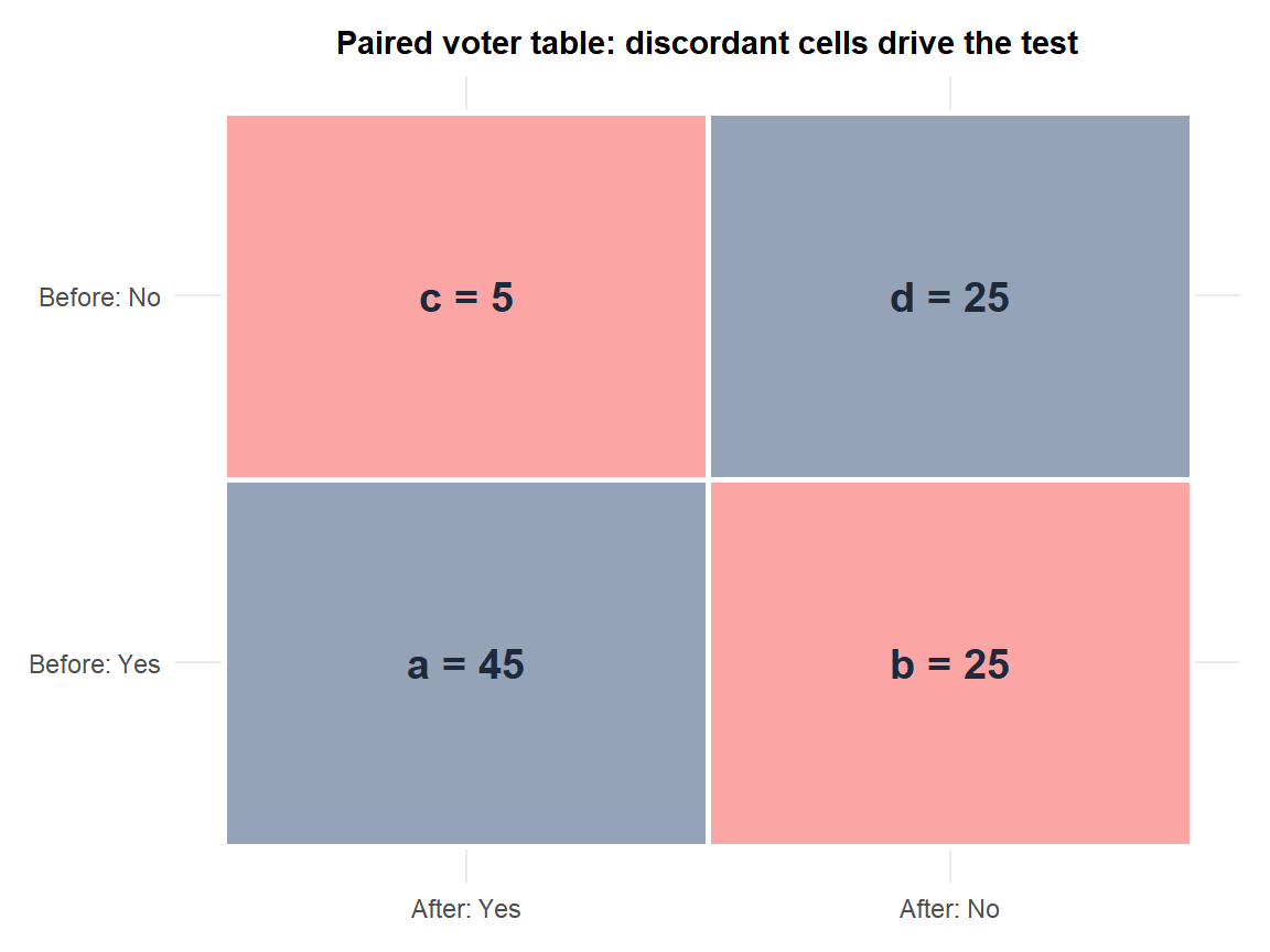
Every subject’s before/after answers land in exactly one of four cells, and only two of them turn out to matter:
| After: Yes | After: No | |
|---|---|---|
| Before: Yes | \(a\) | \(b\) |
| Before: No | \(c\) | \(d\) |
McNemar’s test uses only the discordant pairs, \(b\) (switched from Yes to No) and \(c\) (switched from No to Yes). The concordant pairs \(a\) and \(d\) (people who did not change) carry no information about whether the change is asymmetric, so they drop out of the test entirely.
\[H_0: b = c \text{ (in the population)} \qquad H_1: b \neq c\]
Test statistic, with continuity correction (the standard default):
\[\chi^2 = \frac{(|b-c|-1)^2}{b+c}\]
Without continuity correction:
\[\chi^2 = \frac{(b-c)^2}{b+c}\]
Under \(H_0\), both versions follow a \(\chi^2\) distribution with 1 degree of freedom.
Worked example
A before/after survey on the same voters is the classic setting where treating the two measurements as independent would badly misrepresent what changed:
The same 100 voters are surveyed before and after watching a debate, asked whether they support Candidate A:
| After: Yes | After: No | Total | |
|---|---|---|---|
| Before: Yes | 45 | 25 | 70 |
| Before: No | 5 | 25 | 30 |
| Total | 50 | 50 | 100 |
Discordant pairs: \(b=25\) (supported before, opposed after, lost support) and \(c=5\) (opposed before, supported after, gained support). The 45 steady supporters and 25 steady opposers, the concordant cells \(a\) and \(d\), play no role in the test itself.
Without correction:
\[\chi^2 = \frac{(25-5)^2}{25+5} = \frac{400}{30} = 13.333\]
\(df=1\), \(p = 0.000261\).
With continuity correction:
\[\chi^2 = \frac{(|25-5|-1)^2}{30} = \frac{361}{30} = 12.033\]
\(df=1\), \(p = 0.000523\).
Decision: reject \(H_0\) at any conventional level, whichever version is used. The debate produced a significant net shift in support, specifically a shift away from Candidate A, since far more voters moved from supporting to opposing (25) than the reverse (5), even though the marginal totals (70 vs 50 support before, but only 50 vs 50 after) might at a glance suggest something less dramatic than what the pairing reveals.

When discordant pairs are few
Since the whole test rests on \(b\) and \(c\) alone, a small discordant count breaks the chi-square approximation the same way it does for the ordinary chi-square test:
⚠️ McNemar's test needs enough discordant pairs to be valid
With a small number of discordant pairs (a common rule of thumb: \(b+c < 25\)), the chi-square approximation is unreliable, just like the ordinary chi-square test’s small-expected-frequency problem. In that case use the exact binomial version instead: under \(H_0\), \(b \sim \text{Binomial}(b+c, 0.5)\), and the exact p-value comes directly from the binomial distribution rather than the chi-square approximation. mcnemar.test() does not provide this exact version directly, use binom.test(b, b+c, p = 0.5) on the discordant counts instead when \(b+c\) is small.
Extending beyond 2 categories: the Stuart-Maxwell test
When the paired variable has more than two categories, not just Yes/No, the generalization of McNemar’s test is the Stuart-Maxwell test, or Bowker’s test of symmetry for the general \(r \times r\) case. It tests whether the full table is symmetric across its diagonal. This is not covered in depth here, but it is worth knowing the name exists for when a paired outcome has three or more categories.
Running the test in R
mcnemar.test() takes the 2x2 table directly, and the exact binomial version from above needs only the two discordant counts:
tab <- matrix(c(45, 25, 5, 25), nrow = 2, byrow = TRUE,
              dimnames = list(Before = c("Yes","No"), After = c("Yes","No")))

mcnemar.test(tab)                 # with continuity correction (default)
mcnemar.test(tab, correct = FALSE)

# Exact binomial version for small discordant counts
binom.test(25, 25 + 5, p = 0.5)
💡 McNemar vs chi-square vs paired t-test: which to use
Two independent groups, categorical outcome: use the chi-square test of independence. Same subjects measured twice, categorical/binary outcome: use McNemar’s test, this post. Same subjects measured twice, continuous/numeric outcome: use the paired t-test. The common thread across all three: whenever observations are paired or matched by design, use a method that exploits that pairing, never treat paired data as if it came from independent groups.

