Multicollinearity and VIF

Multicollinearity is when two or more predictors in a multiple regression are highly linearly correlated with each other. It does not bias predictions or hurt overall model fit, but it inflates the standard errors of the affected coefficients, making individual coefficients unstable and their significance tests unreliable. This post builds on the brief mentions in multiple linear regression and regression diagnostics.

Why multicollinearity is a problem

With correlated predictors, the regression cannot cleanly separate each predictor’s individual effect on the response. Small changes in the data can swing the estimated coefficients wildly, standard errors blow up, and coefficient signs can even flip to something implausible, even though the model’s overall predictions stay accurate. The fitted values \(\hat y\) remain trustworthy; it is the individual coefficients, and any story you try to tell from them, that become unreliable.

The Variance Inflation Factor

For predictor \(j\), regress it on all the OTHER predictors and take the resulting \(R_j^2\):

If predictor \(j\) is completely uncorrelated with the others, \(R_j^2 = 0\) and \(VIF_j = 1\): no inflation at all. As \(R_j^2 \to 1\) (predictor \(j\) is almost perfectly explained by a linear combination of the others), \(VIF_j \to \infty\).

The direct interpretation: \(VIF_j\) tells you the coefficient’s variance is \(VIF_j\) times larger than it would be if predictor \(j\) were uncorrelated with the other predictors. Equivalently, the standard error is inflated by a factor of \(\sqrt{VIF_j}\).

Worked example: predicting salary

The clearest way to see multicollinearity is to build a regression where the predictors are deliberately entangled with each other and watch what happens to the coefficients.

Predicting salary with three correlated predictors

A dataset of \(n=50\) employees predicts salary from three predictors that are deliberately correlated: years of experience, age, and years since graduation. In this simulated sample, age and years-since-graduation both move almost in lockstep with experience.

Correlation matrix between the predictors:

	experience	age	grad_years
experience	1.000	0.975	0.968
age	0.975	1.000	0.995
grad_years	0.968	0.995	1.000

All three pairwise correlations are above 0.96, a strong warning sign on its own even before computing VIF.

Regression coefficients from lm(salary ~ experience + age + grad_years):

Predictor	Estimate	Std. Error	t value	p-value
Intercept	15561	9908	1.57	0.123
experience	1246	192	6.50	< 0.001
age	772	453	1.71	0.095
grad_years	-276	418	-0.66	0.512

Overall fit is excellent: \(R^2 = 0.974\), \(F(3,46) = 576\), \(p < 0.001\). Yet only experience is clearly significant; age is borderline and grad_years is not significant at all, and its coefficient even has the wrong sign (negative, implying more years since graduation somehow lowers predicted salary, which makes no substantive sense). This is the classic multicollinearity signature: a strong, significant model overall, but unstable, hard-to-trust individual coefficients.

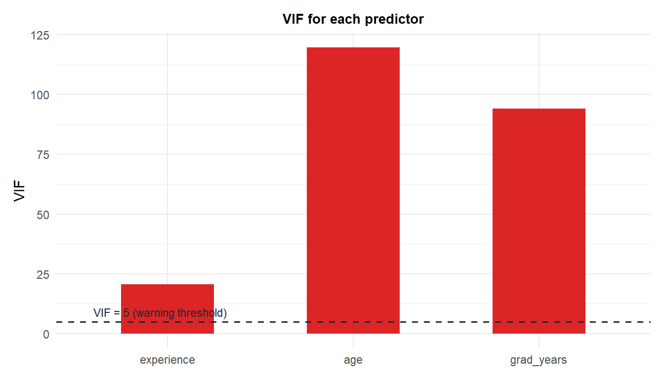
VIF values:

Predictor	VIF
experience	20.6
age	119.7
grad_years	94.1

All three are far above the common rule-of-thumb warning threshold of 5. age’s VIF of 119.7 means its coefficient’s variance is about 120 times larger, and its standard error about \(\sqrt{119.7} \approx 10.9\) times larger, than it would be if age were uncorrelated with experience and grad_years.

Detecting multicollinearity

Besides computing VIF directly, look for:

• A correlation matrix or correlation heatmap of the predictors, as a quick first check, exactly as shown above.
• A high overall \(R^2\) or significant F-test combined with few or no individually significant coefficients, a classic red flag, exactly what happened in the example above.
• Coefficients with an implausible sign or magnitude, as seen with grad_years above.

Fixing multicollinearity

• Drop one of the highly correlated predictors, keeping the one more directly relevant or more reliably measured. Here, experience is probably the most directly meaningful and least redundant of the three.
• Combine correlated predictors into a single index, or use dimensionality reduction such as principal component regression, see principal component analysis.
• Use regularization: ridge regression specifically handles correlated predictors well by shrinking coefficients, see ridge regression.
• Collect more data, or data with more independent variation in the predictors, when feasible.

Running it in R

The full workflow, from fitting the model to checking VIF and the raw correlation matrix, takes just a few lines:

fit <- lm(salary ~ experience + age + grad_years)
summary(fit)

library(car)
vif(fit)

# Correlation matrix of predictors as a quick first check
cor(data.frame(experience, age, grad_years))