t-SNE and UMAP
t-SNE and UMAP are nonlinear dimensionality reduction methods designed for visualization. Unlike PCA, which finds a linear projection that maximizes variance, they preserve the local neighborhood structure of the data: points that are close in high-dimensional space remain close in 2D. The result is a map that reveals clusters, manifold structure, and subpopulations invisible in a PCA plot.
Why PCA is not enough for visualization
PCA is a linear projection: it finds the best flat 2D plane through the high-dimensional data. If the data lies on a curved manifold (e.g., a Swiss roll, a sphere, or a collection of clusters connected by thin bridges), the linear projection crushes the structure and overlaps distant regions.
t-SNE and UMAP learn a nonlinear mapping that “unfolds” the manifold, separating regions that are genuinely different in high dimensions even if they project to the same region under PCA.
t-SNE: t-distributed Stochastic Neighbor Embedding
t-SNE (van der Maaten and Hinton, 2008) converts distances into probabilities separately in the high-dimensional and low-dimensional spaces, then minimizes the KL divergence between them.
In the high-dimensional space: define a Gaussian similarity between points \(i\) and \(j\):
\[p_{j|i} = \frac{\exp(-\|x_i - x_j\|^2 / 2\sigma_i^2)}{\sum_{k \neq i} \exp(-\|x_i - x_k\|^2 / 2\sigma_i^2)}, \quad p_{ij} = \frac{p_{j|i} + p_{i|j}}{2n}\]
The bandwidth \(\sigma_i\) is set so that the effective number of neighbors (perplexity) is approximately the user-specified perplexity parameter.
In the low-dimensional space: use a Student-t distribution with 1 degree of freedom (heavier tails than Gaussian):
\[q_{ij} = \frac{(1 + \|y_i - y_j\|^2)^{-1}}{\sum_{k \neq l}(1 + \|y_k - y_l\|^2)^{-1}}\]
Objective: minimize the KL divergence \(\text{KL}(P \| Q) = \sum_{ij} p_{ij} \log(p_{ij}/q_{ij})\) via gradient descent.
Why the t-distribution? A Gaussian in low dimensions is too concentrated: moderately distant points in high dimensions would all need to be packed close together in 2D (the crowding problem). The heavy tails of the t-distribution allow moderately similar points to be placed farther apart, giving clusters room to breathe.
UMAP: Uniform Manifold Approximation and Projection
UMAP (McInnes et al., 2018) is built on a different mathematical foundation (fuzzy simplicial sets and Riemannian geometry) but shares the same high-level idea: preserve neighborhood structure. Key differences from t-SNE:
- Faster: \(O(n \log n)\) vs t-SNE’s \(O(n^2)\) (Barnes-Hut approximation).
- Better global structure: UMAP attempts to preserve both local and global relationships, not just local ones.
- More stable: less sensitive to random initialization; multiple runs give more similar results.
- General purpose: can project to arbitrary dimensions, not just 2D.
UMAP constructs a fuzzy topological representation of the data, finds a low-dimensional representation with a similar topological structure, and optimizes the cross-entropy between the two fuzzy sets.
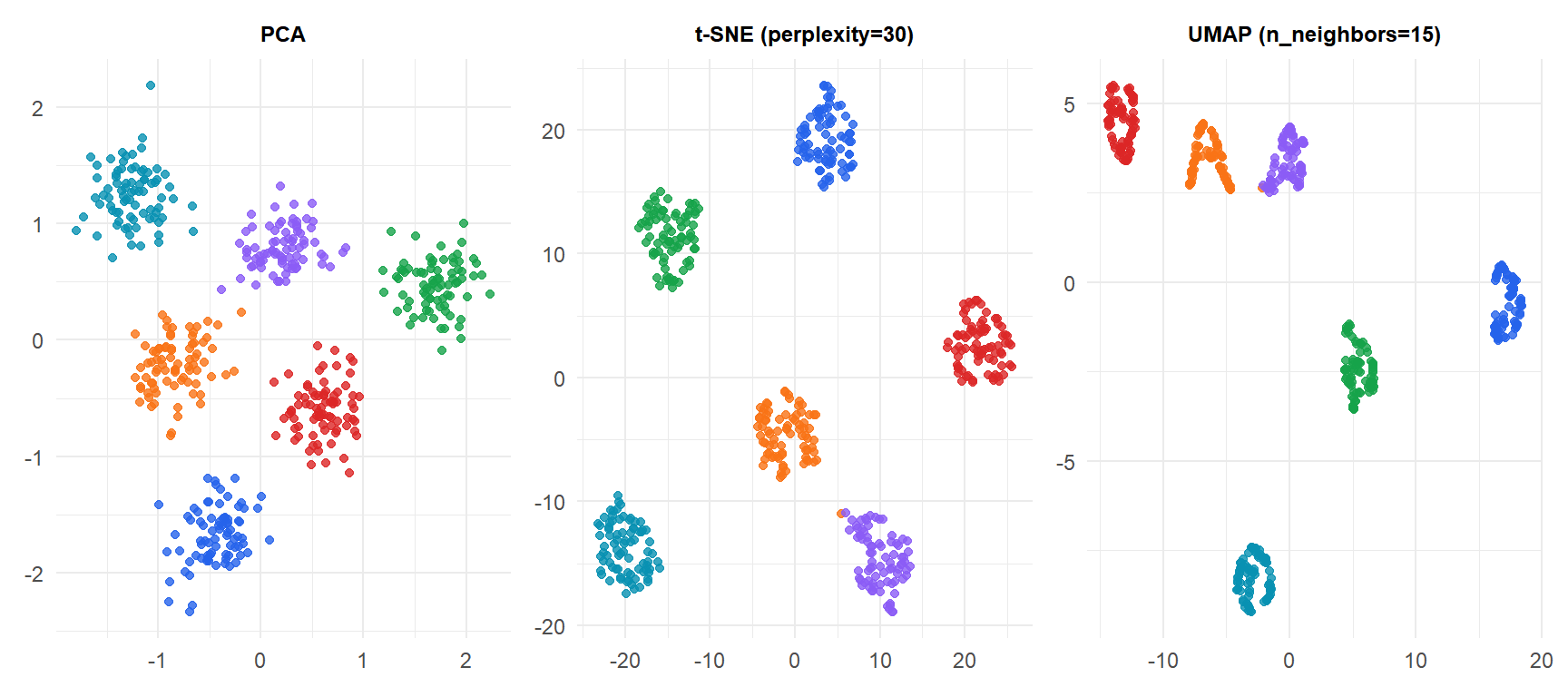
All three methods correctly separate the six clusters on this simple 2D dataset. The advantage of t-SNE and UMAP becomes clear with high-dimensional data (e.g., images, genomics, single-cell RNA-seq) where PCA overlaps distinct subpopulations.
Key hyperparameters
t-SNE: perplexity
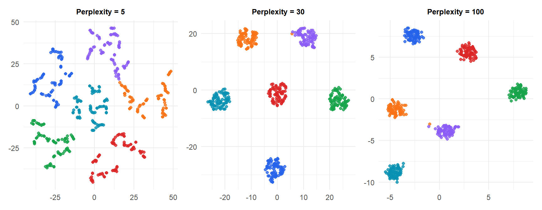
Perplexity controls the effective number of neighbors each point considers. It roughly balances attention between local and global structure:
- Low perplexity (5-10): very local, tight clusters, may fragment large clusters into subclusters.
- High perplexity (50-100): more global, clusters may merge.
- Typical range: 5 to 50. Default: 30.
Rule of thumb: perplexity should be less than \(n/3\).
UMAP: n_neighbors and min_dist
n_neighbors controls the size of the local neighborhood (like perplexity): larger values capture more global structure. min_dist controls how tightly points are packed in the embedding: small values produce tight clusters; large values spread points out more.
Critical pitfalls in interpretation
Both methods produce plots that look like ordinary scatter plots, which tempts people into reading them the way they would read PCA output. That instinct is wrong in several specific, avoidable ways.
⚠️ Four things t-SNE and UMAP plots do NOT tell you
1. Cluster sizes are meaningless. t-SNE expands small dense clusters and compresses large sparse ones. The visual size of a cluster does not reflect the number of points or the spread of the original data.
2. Distances between clusters are not interpretable. t-SNE optimizes local structure; the distance between two well-separated clusters in the 2D plot has no quantitative meaning. Cluster A being twice as far from cluster B as from cluster C does not mean it is twice as different.
3. The number of clusters is not reliable. Both methods can split a single continuous population into apparent subclusters (especially t-SNE with low perplexity) or merge distinct clusters (with high perplexity). Always validate apparent clusters with a clustering algorithm on the original high-dimensional data.
4. Results change with random seed. t-SNE is non-deterministic; each run with a different seed produces a different layout. UMAP is more stable but still varies. Never base conclusions on a single run. For t-SNE, initialize with PCA (pca_init=TRUE) and use multiple seeds.
t-SNE vs UMAP: when to use each
| t-SNE | UMAP | |
|---|---|---|
| Speed | Slow (\(O(n^2)\), Barnes-Hut \(O(n \log n)\)) | Fast (\(O(n \log n)\)) |
| Global structure | Poor | Better |
| Stability | Low (varies by seed) | Higher |
| Scalability | \(n < 100{,}000\) | \(n > 100{,}000\) feasible |
| Interpretability | Very limited | Slightly better |
| Typical use | Biology, single-cell RNA-seq | General purpose, large datasets |
For most new projects: start with UMAP. It is faster, more stable, and preserves more structure. Use t-SNE when comparing with published work that uses it, or in genomics where it is the field standard.
💡 t-SNE and UMAP in R
library(Rtsne)

# t-SNE (remove duplicates first, PCA init for stability)
set.seed(42)
tsne_res <- Rtsne(X, dims=2, perplexity=30, max_iter=1000,
                  pca=TRUE, pca_center=TRUE, normalize=TRUE,
                  check_duplicates=FALSE)
df_tsne <- data.frame(D1=tsne_res$Y[,1], D2=tsne_res$Y[,2])

# UMAP
library(umap)
set.seed(42)
umap_res <- umap(X, n_neighbors=15, min_dist=0.1, n_components=2)
df_umap  <- data.frame(D1=umap_res$layout[,1], D2=umap_res$layout[,2])

# uwot package (faster UMAP, more control)
library(uwot)
embedding <- uwot::umap(X, n_neighbors=15, min_dist=0.1,
                         metric="euclidean", n_epochs=200)
