KKT conditions
The Karush-Kuhn-Tucker (KKT) conditions generalize Lagrange multipliers to problems with inequality constraints. They are the fundamental necessary optimality conditions for constrained optimization: virtually every practical optimization algorithm, from the Simplex method to interior point methods to support vector machines, is built around satisfying the KKT conditions.
The general constrained problem
The KKT conditions are built around this general form, which allows both inequality and equality constraints at the same time:
\[\min_{x \in \mathbb{R}^n} f(x) \quad \text{subject to} \quad g_i(x) \leq 0,\; i=1,\ldots,m \quad h_j(x) = 0,\; j=1,\ldots,p\]
The Lagrangian for this problem is:
\[\mathcal{L}(x, \mu, \lambda) = f(x) + \sum_{i=1}^m \mu_i g_i(x) + \sum_{j=1}^p \lambda_j h_j(x)\]
where \(\mu_i \geq 0\) are the multipliers for inequality constraints and \(\lambda_j\) (unrestricted in sign) are the multipliers for equality constraints.
The five KKT conditions
At a local minimum \(x^*\) satisfying a constraint qualification, there exist multipliers \(\mu^* \geq 0\) and \(\lambda^*\) such that:
1. Stationarity: \[\nabla f(x^*) + \sum_{i=1}^m \mu_i^* \nabla g_i(x^*) + \sum_{j=1}^p \lambda_j^* \nabla h_j(x^*) = \mathbf{0}\]
2. Primal feasibility: \[g_i(x^*) \leq 0 \quad \forall i, \qquad h_j(x^*) = 0 \quad \forall j\]
3. Dual feasibility: \[\mu_i^* \geq 0 \quad \forall i\]
4. Complementary slackness: \[\mu_i^* g_i(x^*) = 0 \quad \forall i\]
Each condition has a clear role:
- Stationarity: the gradient of the Lagrangian is zero. Generalizes the Lagrange condition \(\nabla f = -\lambda \nabla g\) to inequalities.
- Primal feasibility: the solution is feasible. All constraints are satisfied.
- Dual feasibility: inequality multipliers are non-negative. This ensures that active inequality constraints push the solution inward, not outward.
- Complementary slackness: for each inequality constraint, either the constraint is active (\(g_i(x^*) = 0\), constraint boundary is tight) or the multiplier is zero (\(\mu_i^* = 0\), constraint is inactive and plays no role). Both cannot be nonzero simultaneously.
Complementary slackness: the key condition
Complementary slackness is the most distinctive KKT condition. It says that an inactive constraint (one where \(g_i(x^*) < 0\): the solution is strictly inside the feasible region) has no effect on the optimum: \(\mu_i^* = 0\) and the constraint drops out of the stationarity condition.
An active constraint (\(g_i(x^*) = 0\): the solution is on the boundary) may have \(\mu_i^* > 0\): the constraint is binding and its gradient appears in the stationarity condition with nonzero weight.
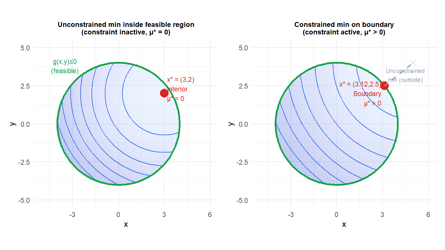
Left: the unconstrained minimum \((3,2)\) lies inside the feasible disk. The constraint is inactive (\(g(x^*)=0^2+2^2-16 = -7 < 0\)), so \(\mu^* = 0\) and the constraint plays no role. Right: the unconstrained minimum \((5,4)\) lies outside the feasible region. The constrained optimum is the projection onto the boundary disk, where the constraint is active (\(g(x^*)=0\)) and \(\mu^* > 0\).
Complete example: inequality-constrained quadratic
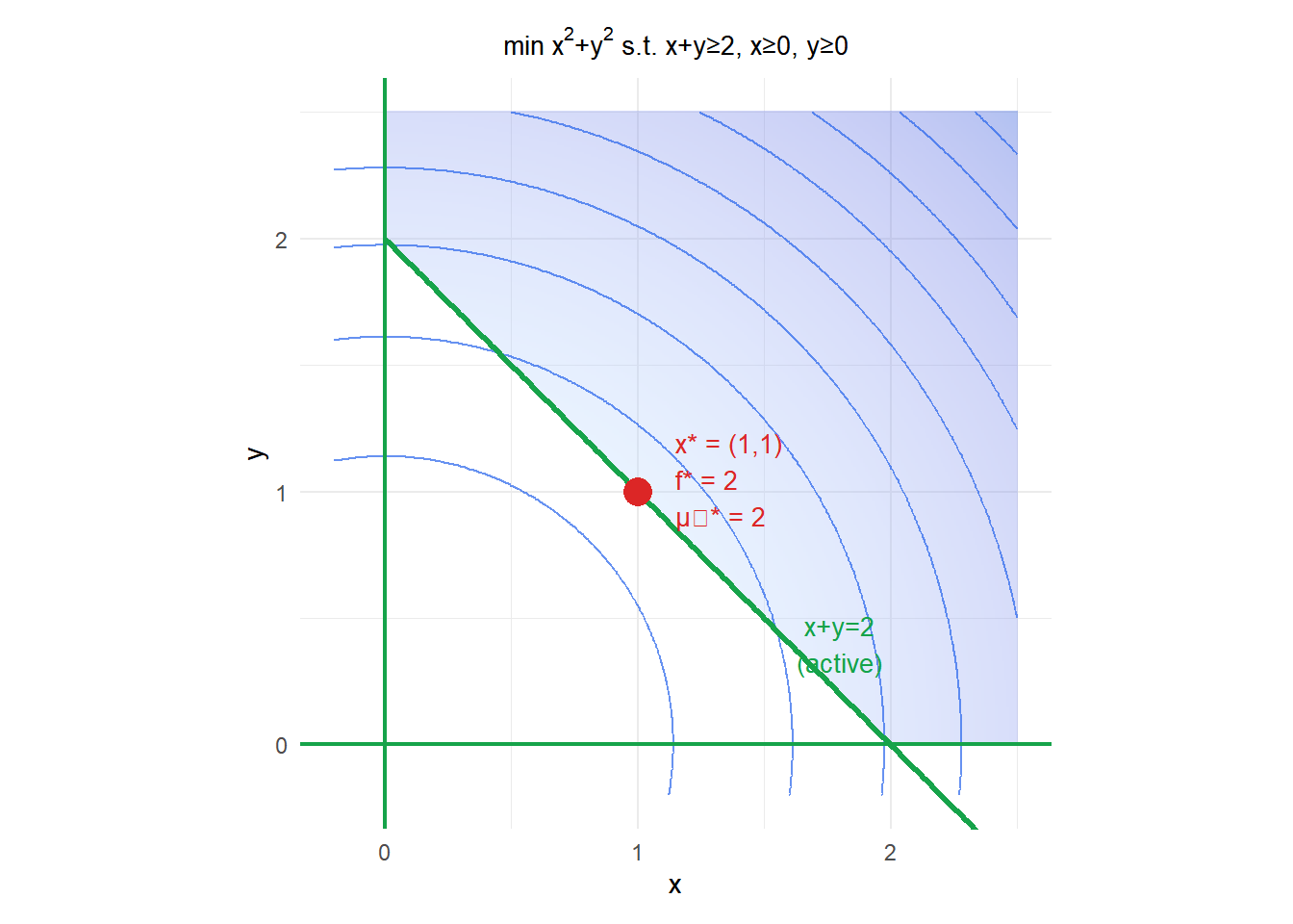
Minimize \(f(x,y) = x^2 + y^2\) subject to \(g_1: x + y \geq 2\) (i.e., \(2 - x - y \leq 0\)) and \(g_2: x \geq 0\), \(g_3: y \geq 0\).
Rewrite in standard form (\(g_i \leq 0\)): \(g_1 = 2-x-y\), \(g_2 = -x\), \(g_3 = -y\).
Lagrangian:
\[\mathcal{L} = x^2 + y^2 + \mu_1(2-x-y) + \mu_2(-x) + \mu_3(-y)\]
Stationarity:
\[2x - \mu_1 - \mu_2 = 0 \implies \mu_1 + \mu_2 = 2x\]
\[2y - \mu_1 - \mu_3 = 0 \implies \mu_1 + \mu_3 = 2y\]
By symmetry (\(f\) and the binding constraint \(x+y=2\) are symmetric), try \(x^* = y^* = 1\).
Check: \(g_1 = 2-1-1=0\) (active), \(g_2 = -1 < 0\) (inactive, so \(\mu_2=0\)), \(g_3 = -1 < 0\) (inactive, so \(\mu_3=0\)).
From stationarity with \(\mu_2=\mu_3=0\): \(\mu_1 = 2x^* = 2\). Check dual feasibility: \(\mu_1=2 > 0\). Check complementary slackness: \(\mu_1 g_1 = 2 \times 0 = 0\), \(\mu_2 g_2 = 0 \times (-1) = 0\), \(\mu_3 g_3 = 0 \times (-1) = 0\). All satisfied.
Optimal solution: \(x^* = y^* = 1\), \(f^* = 2\), \(\mu_1^* = 2\).
The multiplier \(\mu_1^* = 2\) tells us: tightening the constraint from \(x+y \geq 2\) to \(x+y \geq 2+\varepsilon\) increases the optimal value by approximately \(2\varepsilon\).
Sufficiency: when KKT implies global optimality
KKT conditions are always necessary (under a constraint qualification). They are sufficient for global optimality when:
- \(f\) is convex.
- Each \(g_i\) is convex (so \(g_i(x) \leq 0\) defines a convex feasible set).
- Each \(h_j\) is affine (linear).
Under these conditions, any KKT point is a global minimum. This covers the most important practical cases: linear programming, quadratic programming with convex objective, convex portfolio optimization, support vector machines.
For non-convex problems, KKT points may be local minima, local maxima, or saddle points. Finding the global minimum requires additional structure or global search methods.
Application: support vector machines
SVMs find the maximum-margin hyperplane separating two classes. The primal problem is:
\[\min_{w,b} \frac{1}{2}\|w\|^2 \quad \text{s.t.} \quad y_i(w^T x_i + b) \geq 1 \quad \forall i\]
The KKT conditions give the dual problem: only support vectors (points where \(\mu_i > 0\), i.e., the constraint \(y_i(w^T x_i+b) = 1\) is active) appear in the solution. Points far from the margin have \(\mu_i = 0\) by complementary slackness and are irrelevant. This sparsity is a direct consequence of KKT.
⚠️ KKT conditions require constraint qualification
The most common constraint qualification is Linear Independence CQ (LICQ): the gradients of the active constraints at \(x^*\) must be linearly independent. If LICQ fails, KKT multipliers may not exist or may not be unique.
Common situations where CQ can fail:
- Two inequality constraints are tangent to each other at the optimum.
- A constraint has zero gradient at the optimum.
- Too many active constraints (more than \(n\) active constraints in \(\mathbb{R}^n\)).
In practice, CQ failure is rare in well-posed problems. If you suspect it, check that the active constraint gradients are linearly independent at your candidate optimum.
💡 Checking KKT conditions in practice
Given a candidate point \(x^*\), verify KKT manually:
- Check primal feasibility: all \(g_i(x^*) \leq 0\) and \(h_j(x^*) = 0\).
- Compute \(\nabla f(x^*)\) and \(\nabla g_i(x^*)\) for active constraints.
- Solve the linear system for \(\mu_i^*\) from the stationarity condition.
- Check dual feasibility: \(\mu_i^* \geq 0\) for all \(i\).
- Check complementary slackness: \(\mu_i^* g_i(x^*) = 0\) for all \(i\).
In R, numerical KKT verification after solving with nloptr:
library(nloptr)

f      <- function(x) x[1]^2 + x[2]^2
grad_f <- function(x) c(2*x[1], 2*x[2])
g_ineq <- function(x) c(2 - x[1] - x[2], -x[1], -x[2])

res <- nloptr(x0=c(0.5, 0.5), eval_f=f, eval_grad_f=grad_f,
              eval_g_ineq=g_ineq,
              opts=list(algorithm="NLOPT_LD_SLSQP", xtol_rel=1e-8))
res$solution  # c(1, 1)
