Markov chains
A Markov chain models a system that moves between a set of states over time, where the probability of moving to the next state depends only on the current state, not on how the system got there. This “no memory of the past” property makes Markov chains one of the simplest and most useful models of random processes that unfold over time, and it builds directly on the random experiments covered earlier in this section.
The Markov property
For a sequence of states \(X_0, X_1, X_2, \ldots\), the Markov property says:
\[P(X_{n+1} = j \mid X_n = i, X_{n-1}, \ldots, X_0) = P(X_{n+1} = j \mid X_n = i)\]
Everything relevant about the future is already captured by the present state. The entire past history adds nothing extra once you know where the system is right now.
The transition matrix
Collect the one-step transition probabilities \(p_{ij} = P(X_{n+1}=j \mid X_n=i)\) into a matrix \(P\). Each row of \(P\) must sum to 1: from state \(i\), the system has to go somewhere, possibly staying in \(i\).
Worked example: a simple weather model
A two-state system is the easiest place to see the transition matrix and the long-run stationary distribution in action.
Two states, Sunny and Rainy. If today is sunny, tomorrow is sunny with probability 0.8 and rainy with probability 0.2. If today is rainy, tomorrow is sunny with probability 0.4 and rainy with probability 0.6. The transition matrix (rows and columns ordered Sunny, Rainy):
\[P = \begin{pmatrix} 0.8 & 0.2 \\ 0.4 & 0.6 \end{pmatrix}\]
Starting from a sunny day ($X_0 = $ Sunny, so the initial distribution is \((1, 0)\)), find the probability distribution over the next few days by repeatedly multiplying by \(P\).
Day 1: \((1,0) \cdot P = (0.8,\ 0.2)\).
Day 2: \((0.8, 0.2) \cdot P = (0.8 \times 0.8 + 0.2 \times 0.4,\ \ 0.8 \times 0.2 + 0.2 \times 0.6) = (0.64+0.08,\ \ 0.16+0.12) = (0.72,\ 0.28)\).
Day 3: \((0.72, 0.28) \cdot P = (0.688,\ 0.312)\).
So the probability of a sunny day is \(0.8 \to 0.72 \to 0.688\), slowly drifting downward day by day, even though today was guaranteed sunny.

The stationary distribution
As \(n \to \infty\), the distribution over states settles down to a fixed long-run distribution \(\pi\) that no longer changes from one step to the next.
\[\pi P = \pi, \qquad \sum_i \pi_i = 1\]
\(\pi\) is a left eigenvector of \(P\) with eigenvalue 1, normalized so its entries sum to 1.
For the weather example, the stationary distribution is \(\pi = (2/3,\ 1/3) = (0.6667,\ 0.3333)\): in the long run, about two-thirds of days are sunny and one-third rainy, regardless of what today’s weather is. This matches the trend already visible in the day-by-day sequence above: \(0.8 \to 0.72 \to 0.688\) is slowly converging down toward \(0.6667\).
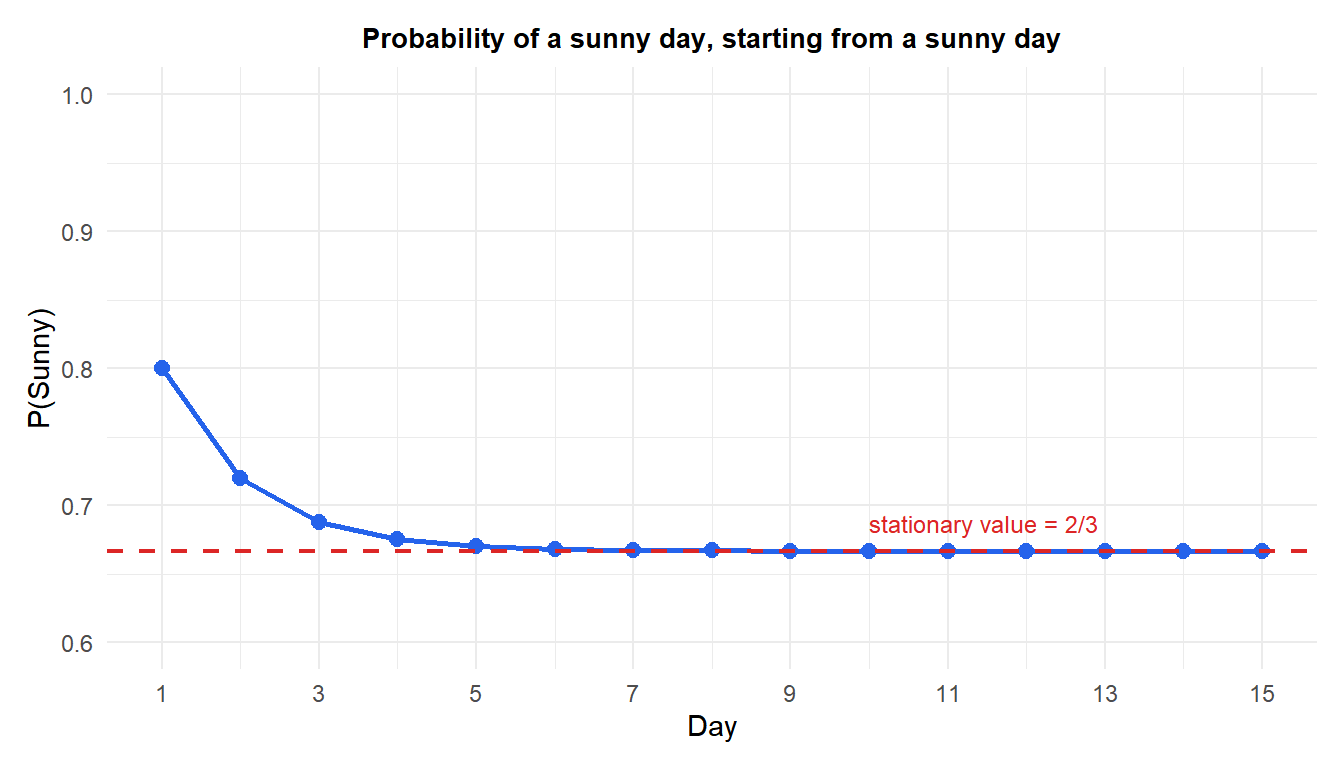
The probability of a sunny day decays smoothly and monotonically from 1 down toward the stationary value \(2/3\), regardless of the fact that day 0 was certainly sunny.
Finding the stationary distribution in R
Solving \(\pi P = \pi\) is equivalent to finding the left eigenvector of \(P\) associated with eigenvalue 1 (equivalently, the eigenvector of \(P^T\) for eigenvalue 1), then normalizing it to sum to 1.
⚠️ A stationary distribution only exists, and is unique, under conditions
Not every Markov chain has a unique stationary distribution. It requires the chain to be irreducible (every state reachable from every other state) and aperiodic (it doesn’t cycle through states in a rigid, predictable pattern). The weather example satisfies both trivially: you can reach either state from either state, and there is no forced cycle. But chains with absorbing states (a state you can enter but never leave) or chains that strictly alternate between states in a fixed cycle can fail to converge to a single stationary distribution, or can have one but never actually reach it from every starting point.
Where Markov chains show up
The abstract math grounds a surprising range of real applications:
- Google’s PageRank: web pages as states, links as transitions, the stationary distribution ranks page importance.
- Markov Chain Monte Carlo (MCMC): used throughout Bayesian computation to sample from complex posterior distributions.
- Text generation and autocomplete: word-to-word (or character-to-character) transition probabilities.
- Board games and queueing models: dice-driven position changes, customers arriving and leaving a queue.
- Genetics: modeling sequences of nucleotides along a strand of DNA.
Running it in R
The weather model above, its multi-step transitions and its stationary distribution all come from a handful of matrix operations:
P <- matrix(c(0.8, 0.2,
              0.4, 0.6), nrow = 2, byrow = TRUE)
rownames(P) <- colnames(P) <- c("Sunny", "Rainy")

# n-step transition: probability distribution after n days starting Sunny
library(expm)
p0 <- c(1, 0)
p0 %*% (P %^% 3)

# Stationary distribution via eigenvectors
ev <- eigen(t(P))
pi_vec <- Re(ev$vectors[, which(abs(ev$values - 1) < 1e-8)])
pi_vec / sum(pi_vec)

# Simulate a random walk through the chain
library(markovchain)
mc <- new("markovchain", states = c("Sunny","Rainy"), transitionMatrix = P)
rmarkovchain(n = 20, object = mc, t0 = "Sunny")
💡 Reading a transition matrix quickly
Rows are “from”, columns are “to”, and every row must sum to exactly 1, a quick sanity check when building or inspecting a transition matrix by hand. The diagonal entries \(p_{ii}\) tell you how “sticky” a state is: how likely the system is to stay put rather than transition away. In the weather example, Sunny is stickier (0.8) than Rainy (0.6), which is exactly why the long-run stationary distribution favors sunny days.

