STL decomposition
Any time series can be understood as the sum of a handful of simpler pieces: an underlying trend, a repeating seasonal pattern, and whatever is left over. STL decomposition (Seasonal-Trend decomposition using Loess) is the standard, robust way to split a series into exactly these three components. This post builds on the components introduced in what is a time series?, and pairs naturally with checking stationarity, since removing trend and seasonality is often the first step toward a stationary series.
The additive decomposition model
Every observation is simply the sum of its three underlying pieces:
\[y_t = T_t + S_t + R_t\]
where \(T_t\) is the trend component (the slow-moving underlying level), \(S_t\) is the seasonal component (a pattern that repeats at a fixed, known period, e.g. every 12 months), and \(R_t\) is the remainder (whatever the trend and seasonal components don’t explain).
There is also a multiplicative alternative, \(y_t = T_t \times S_t \times R_t\), used when the seasonal swings grow proportionally with the series’ level rather than staying a constant absolute size. It is equivalent to running an additive decomposition on \(\log(y_t)\).
Classical decomposition: the simpler baseline
The older decompose()-style approach works in two steps: estimate the trend with a moving average whose window equals the seasonal period, subtract it out, then average the detrended values within each seasonal position (e.g. average all Januaries together) to get a single, fixed, repeating seasonal component. Whatever remains after removing both is the remainder.
This has two real weaknesses, both of which STL fixes:
- The trend estimate loses the first and last half-period of observations, a centered moving average needs data on both sides, so it cannot be computed right at the edges of the series.
- The seasonal component is forced to be perfectly identical in every cycle, it cannot change gradually over time. A real seasonal pattern that gently drifts, for instance summer sales becoming more dominant year after year, cannot be captured at all.
STL: what makes it different
STL replaces the moving-average trend and the fixed seasonal average with local regression (LOESS) smoothing for both components, applied iteratively. This gives two concrete advantages over classical decomposition:
- The seasonal component is allowed to slowly change shape over time instead of being frozen into one repeating cycle.
- STL is robust to outliers: an unusually extreme observation can be down-weighted so it doesn’t drag the whole trend or seasonal estimate off course, ending up isolated in the remainder instead.
Worked example: decomposing 6 years of monthly sales
Simulating a series with a known trend and a known seasonal shape built in makes it possible to check that STL actually recovers both pieces, and how little is left over in the remainder.
Simulated monthly sales data, 72 months (6 years), with a rising trend, a clear yearly seasonal cycle, and noise:
set.seed(3)
n_months <- 72
t <- 1:n_months
trend <- 500 + 8*t
seasonal <- 150*sin(2*pi*t/12) + 60*cos(2*pi*t/12)
noise <- rnorm(n_months, 0, 40)
y <- trend + seasonal + noise
ts_y <- ts(y, frequency = 12, start = c(2019, 1))
fit_stl <- stl(ts_y, s.window = "periodic")
First-year (12 months) actual values and the resulting STL components:
| Month | \(y_t\) (sales) | Trend \(T_t\) | Seasonal \(S_t\) | Remainder \(R_t\) |
|---|---|---|---|---|
| 1 | 596.48 | 497.10 | 119.52 | -20.14 |
| 2 | 664.20 | 505.96 | 152.40 | 5.84 |
| 3 | 684.35 | 514.82 | 157.62 | 11.91 |
| 4 | 585.82 | 523.43 | 97.48 | -35.09 |
| 5 | 570.87 | 532.03 | 31.88 | 6.96 |
| 6 | 489.20 | 540.49 | -87.32 | 36.04 |
| 7 | 432.46 | 548.94 | -110.15 | -6.34 |
| 8 | 448.76 | 557.41 | -142.95 | 34.30 |
| 9 | 373.25 | 565.88 | -164.35 | -28.29 |
| 10 | 530.79 | 573.61 | -91.43 | 48.61 |
| 11 | 535.17 | 581.35 | -20.49 | -25.69 |
| 12 | 610.75 | 588.52 | 57.77 | -35.55 |
The additive identity holds exactly, for month 1: \(497.10 + 119.52 - 20.14 = 596.48\).
Over the full 72 months, the trend rises from about 497 to 1072, the seasonal component ranges from about -164 to +158 (a clear yearly cycle peaking around March and bottoming around September), and the remainder has standard deviation 31.1. The trend and seasonal components together explain about 97.6% of the total variance in the series (remainder variance 965.8 out of total variance 39782.2), only 2.4% is left unexplained noise, confirming the decomposition captured the two systematic patterns well.

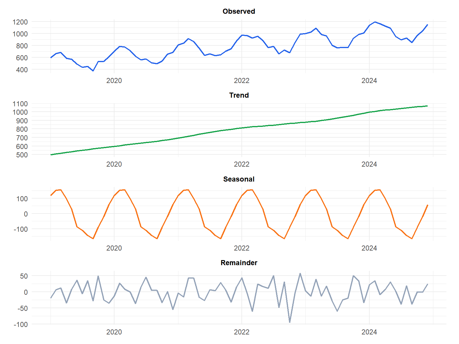
The trend (green) rises smoothly and steadily. The seasonal component (orange) repeats every 12 months with a stable shape. The remainder (grey) has no visible pattern left, exactly what a good decomposition should leave behind.
⚠️ A large or patterned remainder means the decomposition missed something
The remainder should look like unstructured noise: no visible trend, no repeating pattern, no clusters of unusually large residuals. If the remainder still shows a clear pattern, a leftover slow drift, or larger swings during certain months every year, it usually means the seasonal period was mis-specified, there’s a second seasonal cycle the model isn’t capturing (for instance both a weekly AND a yearly pattern in daily data), or there’s a structural break, a sudden regime change, that a smooth decomposition simply cannot represent.
Always plot the remainder and inspect it. Don’t just trust that the trend and seasonal panels look reasonable.
Choosing the seasonal window (s.window)
The s.window argument controls how much the seasonal component is allowed to change over time. s.window = "periodic", used in the example above, forces a perfectly fixed, unchanging seasonal pattern, equivalent to classical decomposition’s seasonal step. It is a good, safe default when there’s no reason to expect the seasonal pattern itself to evolve.
A numeric odd value, for instance s.window = 7, instead allows the seasonal shape to drift slowly over time, useful for series where the seasonal pattern genuinely changes across years.
Running it in R
The whole decomposition above, from building the ts object to extracting each component, comes down to a couple of function calls:
ts_y <- ts(y, frequency = 12, start = c(2019, 1))

# STL decomposition
fit_stl <- stl(ts_y, s.window = "periodic")
plot(fit_stl)
components <- fit_stl$time.series   # matrix with seasonal, trend, remainder columns

# Classical decomposition for comparison
fit_classical <- decompose(ts_y, type = "additive")
plot(fit_classical)

# Seasonally adjusted series (original minus the seasonal component)
seasonally_adjusted <- ts_y - components[, "seasonal"]
💡 STL vs classical decomposition: which to use
Use STL by default. It handles a changing seasonal pattern, is robust to outliers, and doesn’t lose observations at the start and end of the series the way classical decomposition’s moving average does. Classical decomposition is mainly useful today as a simple, quick first look, or when a downstream tool specifically expects its output format.
STL only handles a single seasonal period at a time (the frequency set in the ts object). For series with multiple seasonal cycles, for instance both weekly and yearly patterns in daily data, use mstl() from the forecast package instead, which extends STL to multiple seasonalities.

