Multinomial distribution
The multinomial distribution generalizes the binomial distribution from two outcomes per trial to any fixed number of categories. Across \(n\) independent trials, each landing in exactly one of \(k\) categories with fixed probabilities, it gives the joint probability of observing any particular combination of category counts.
Definition
A random vector \((X_1, X_2, \ldots, X_k)\) follows a multinomial distribution with parameters \(n\) (number of trials) and \(p_1, p_2, \ldots, p_k\) (category probabilities, summing to 1), written \((X_1,\ldots,X_k) \sim \text{Multinomial}(n, p_1,\ldots,p_k)\), if:
\[P(X_1=x_1,\ldots,X_k=x_k) = \frac{n!}{x_1!\, x_2! \cdots x_k!}\, p_1^{x_1} p_2^{x_2} \cdots p_k^{x_k}, \quad \sum_{i=1}^k x_i = n\]
Each \(X_i\) counts how many of the \(n\) trials landed in category \(i\). The counts are not free to vary independently: because every trial lands in exactly one category, they must always add up to the fixed total \(n\). When \(k=2\), this reduces exactly to the binomial distribution, with \(X_1\) the usual “number of successes” and \(X_2 = n - X_1\) the number of failures.
Properties
For \((X_1,\ldots,X_k) \sim \text{Multinomial}(n, p_1,\ldots,p_k)\):
- Marginal distribution
Each individual \(X_i\), on its own, follows a binomial distribution: \(X_i \sim \text{Binomial}(n, p_i)\). Every trial either falls into category \(i\) (a “success” with probability \(p_i\)) or into some other category (a “failure” with probability \(1-p_i\)), which is exactly the binomial setup.
- Expected value
\[E(X_i) = np_i\]
- Variance
\[\text{Var}(X_i) = np_i(1-p_i)\]
Identical to the binomial variance, since the marginal distribution is binomial.
- Covariance between categories
\[\text{Cov}(X_i, X_j) = -np_ip_j, \quad i \neq j\]
This covariance is always negative. Since every trial lands in exactly one category, the counts compete for the same fixed total \(n\): if more trials than expected land in category \(i\), strictly fewer are left available for category \(j\). The categories cannot move up or down together, so treating them as independent binomials and ignoring this negative correlation gives the wrong joint behavior.
Worked example: customers choosing among three products
Putting a number on both the joint probability of one specific outcome and the negative covariance between categories makes the two properties above concrete.
A company knows that, historically, customers choose between three products A, B and C with probabilities \(p = (0.5,\ 0.3,\ 0.2)\). A sample of \(n=50\) independent customers is observed, and the exact split turns out to be 28 choosing A, 14 choosing B, and 8 choosing C.
The joint probability of this exact split:
\[P(X_A=28, X_B=14, X_C=8) = \frac{50!}{28!\,14!\,8!}(0.5)^{28}(0.3)^{14}(0.2)^{8} \approx 0.0129\]
Looking only at product A on its own, its marginal distribution is \(X_A \sim \text{Binomial}(50, 0.5)\), with \(E(X_A) = 25\) and \(\text{Var}(X_A) = 12.5\). Observing 28 is 3 above the expected count of 25, a single-category probability of \(P(X_A=28) \approx 0.0788\) under that marginal binomial.
The negative covariance shows up immediately in the data: \(\text{Cov}(X_A,X_B) = -50 \times 0.5 \times 0.3 = -7.5\), \(\text{Cov}(X_A,X_C) = -50 \times 0.5 \times 0.2 = -5\), and \(\text{Cov}(X_B,X_C) = -50 \times 0.3 \times 0.2 = -3\). A direct simulation of 200,000 draws from this multinomial confirms it: the empirical covariances come out at \(-7.508\), \(-5.066\) and \(-2.979\), matching the theoretical values closely, and the empirical correlation between \(X_A\) and \(X_B\) alone is about \(-0.654\), a strong negative relationship driven entirely by the fixed-total constraint.

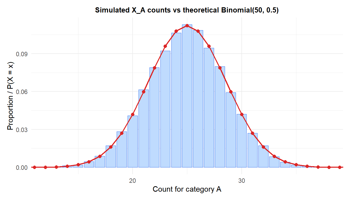
The blue bars are the simulated frequencies of category A’s count across 50,000 independent multinomial draws. The red curve is the exact theoretical \(\text{Binomial}(50, 0.5)\) PMF. They line up essentially perfectly, confirming the marginal property: looking at any single category in isolation, the multinomial behaves exactly like a binomial.
⚠️ The categories are not independent binomials
Each \(X_i\) is individually binomial, but \((X_1,\ldots,X_k)\) jointly is not a set of independent binomials, the negative covariance above is real and ignoring it is a common mistake. This matters most when testing whether observed category counts match a hypothesized set of probabilities: the standard tool is a chi-square goodness-of-fit test, which correctly accounts for the fact that the counts must sum to \(n\), rather than running \(k\) separate one-off binomial tests.
Running it in R
Base R covers the exact probability, the simulation, and the goodness-of-fit test with no extra packages:
p <- c(0.5, 0.3, 0.2)
n <- 50

# Exact joint probability of a specific count vector
dmultinom(c(28, 14, 8), size = n, prob = p)

# Simulate many draws
sims <- t(rmultinom(10000, size = n, prob = p))

# Test observed counts against the hypothesized probabilities
chisq.test(c(28, 14, 8), p = p)
💡 Where the multinomial shows up in practice
Survey responses across more than two answer options, dice rolls across all six faces, word or token counts in a document (the basis of the naive Bayes text classifier), and allele frequencies across more than two genetic variants are all classic multinomial settings. Any time outcomes fall into one of several fixed categories across repeated independent trials, the multinomial is the natural joint distribution for the category counts.

