Confidence interval vs prediction interval
A confidence interval estimates where a population parameter, such as the true mean \(\mu\), actually lies. A prediction interval estimates where a single future observation will fall. The second is always wider, often much wider, because it has to account for both the uncertainty in estimating the parameter and the natural variability of individual observations around it.
The two formulas, side by side
For a sample of size \(n\) from a normal population, with sample mean \(\bar{x}\) and sample standard deviation \(S\):
\[\text{CI for } \mu: \quad \bar{x} \pm t_{\alpha/2,\,n-1} \cdot \frac{S}{\sqrt{n}}\]
\[\text{PI for a new observation}: \quad \bar{x} \pm t_{\alpha/2,\,n-1} \cdot S\sqrt{1 + \frac{1}{n}}\]
The two formulas share the same center and the same critical value \(t_{\alpha/2,\,n-1}\), the only difference is what sits under the square root. The confidence interval’s standard error, \(S/\sqrt{n}\), only captures how precisely \(\bar{x}\) estimates \(\mu\). The prediction interval adds a “+1” inside the square root, which is exactly the extra variance of one new, individual observation around the true mean, a source of uncertainty that has nothing to do with sample size.
That “+1” is the whole story: as \(n \to \infty\), \(S/\sqrt{n} \to 0\) and the confidence interval collapses toward a single point, but \(S\sqrt{1 + 1/n} \to S\), so the prediction interval shrinks only slightly and settles at a floor width set by the population’s own spread. No amount of extra data will ever make a single future observation perfectly predictable.
Worked example: a sample mean
The two intervals start from the exact same sample, the only thing that changes is what question is being asked of it.
A sample of \(n=25\) reaction-time measurements gives \(\bar{x} = 255.63\) ms and \(S = 39.19\) ms. With \(t_{0.025,\,24} = 2.064\):
| Formula | Interval | Width | |
|---|---|---|---|
| 95% CI for \(\mu\) | \(255.63 \pm 2.064 \times 39.19/\sqrt{25}\) | [239.45, 271.80] | 32.35 |
| 95% PI for a new value | \(255.63 \pm 2.064 \times 39.19\sqrt{1+1/25}\) | [173.14, 338.11] | 164.98 |
The prediction interval is about 5.1 times wider than the confidence interval, for the exact same sample. The confidence interval says “the true average reaction time is almost certainly between 239 and 272 ms”. The prediction interval says something much broader: “a single new measurement from this process could plausibly land anywhere from 173 to 338 ms”. Both statements are correct, they are just answering different questions.

The same distinction in regression
The gap between the two intervals is easiest to see in a simple linear regression, where both can be read off the same fitted line at any value of \(x\).
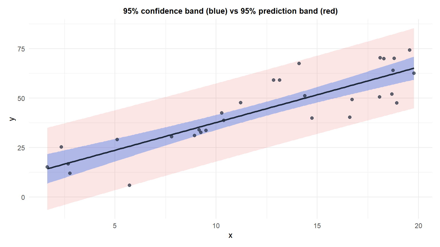
At \(x = 10\), the fitted value is \(\hat{y} = 41.30\): the 95% confidence interval for the mean response is \([38.33, 44.26]\), width 5.93, while the 95% prediction interval for a new individual response is \([25.22, 57.38]\), width 32.16, about 5.4 times wider. The narrow blue band hugs the fitted line tightly almost everywhere; the red band is wide even near the center of the data, because it has to cover where one new point might fall, not just where the average line sits.
Why confusing them is a consequential mistake
Picking the wrong one of the two is not a cosmetic error, it changes how much uncertainty gets reported to whoever is making a decision from it.
⚠️ A narrow confidence interval can create false confidence about one future case
Reporting a confidence interval when a decision depends on a single future observation systematically understates the real uncertainty. A demand forecast with a tight 95% CI around the average next-month sales looks reassuring, but if the actual decision is “how much inventory do we need so we do not run out next month”, the relevant range is the prediction interval for that one month, which can be several times wider. Using the CI there quietly removes most of the real risk from the picture.
Running it in R
For a regression, both intervals come from the same predict() call, just with a different interval argument:
fit <- lm(y ~ x, data = df)

predict(fit, newdata = data.frame(x = 10), interval = "confidence", level = 0.95)
predict(fit, newdata = data.frame(x = 10), interval = "prediction", level = 0.95)
For a plain sample mean (no regression), base R has a one-line function for the confidence interval but not for the prediction interval, which has to be computed from the formula directly:
t.test(x)$conf.int                 # 95% CI for the mean

n <- length(x)
tcrit <- qt(0.975, df = n - 1)
xbar  <- mean(x); s <- sd(x)
pi_lo <- xbar - tcrit * s * sqrt(1 + 1/n)   # 95% PI for a new observation
pi_hi <- xbar + tcrit * s * sqrt(1 + 1/n)
💡 The core takeaway as n grows
As the sample size increases, the confidence interval keeps narrowing toward zero width, you can in principle pin down \(\mu\) as precisely as you like with enough data. The prediction interval does the opposite: it narrows only slightly and converges to a floor set by \(S\), the population’s own variability, which no amount of additional data can shrink away. If the question is about the parameter, more data is the answer. If the question is about one future case, there is a limit to how much more certain you can become.

