Maximum likelihood estimation

Maximum likelihood estimation (MLE) is the most widely used method for estimating a distribution’s parameters: it picks the parameter values that make the data you actually observed as probable as possible. It underlies far more of this site than it might seem, logistic regression is fit by MLE, not by minimizing squared error.

The likelihood function

For independent, identically distributed observations \(x_1, x_2, \ldots, x_n\) from a distribution with parameter \(\theta\) and density or mass function \(f(x;\theta)\), the likelihood is the joint probability of the observed data, viewed as a function of \(\theta\) with the data held fixed:

This is a conceptual flip from how probability usually works. A probability function asks: given these parameters, how likely is this data? A likelihood function asks the reverse: given this data, how does its probability change as the parameters vary? The maximum likelihood estimate \(\hat\theta\) is whichever value of \(\theta\) maximizes \(L(\theta)\).

Why the log-likelihood

Products of many small probabilities underflow numerically and are awkward to differentiate. Taking logs turns the product into a sum without changing where the maximum is, since the logarithm is a strictly increasing function:

\[\ell(\theta) = \log L(\theta) = \sum_{i=1}^n \log f(x_i; \theta)\]

In practice, always maximize \(\ell(\theta)\), never \(L(\theta)\) directly.

Worked example 1: MLE for a Bernoulli proportion

The simplest possible case, a coin flip, already shows the full mechanics: write the likelihood, take the derivative, and solve.

How many coin flips landed heads?

A coin is flipped 10 times, recording 1 for heads and 0 for tails: \(1,0,1,1,0,1,1,1,0,1\) (7 heads out of 10). For i.i.d. Bernoulli(\(p\)) data, the likelihood and log-likelihood are:

\[L(p) = p^{\sum x_i}(1-p)^{n-\sum x_i}, \qquad \ell(p) = \Big(\sum x_i\Big)\log p + \Big(n-\sum x_i\Big)\log(1-p)\]

Take the derivative with respect to \(p\) and set it to zero:

\[\frac{d\ell}{dp} = \frac{\sum x_i}{p} - \frac{n - \sum x_i}{1-p} = 0\]

Solving gives the maximum likelihood estimator:

\[\hat{p}_{MLE} = \frac{\sum x_i}{n}\]

For this data: \(n=10\), \(\sum x_i = 7\), so \(\hat p_{MLE} = 7/10 = 0.7\). This is exactly the sample proportion, the “obvious” estimator turns out to be the maximum likelihood estimator.

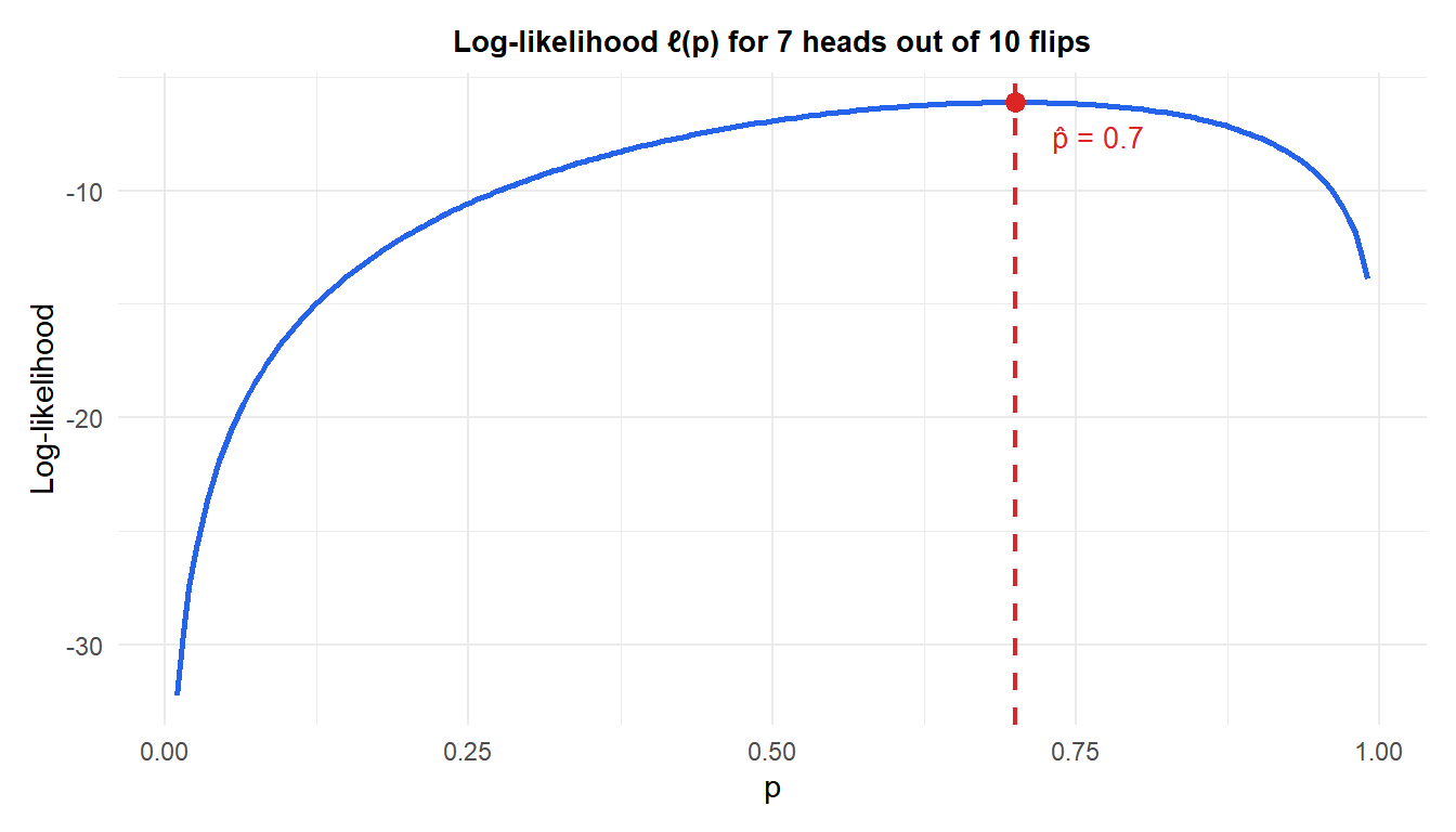
The curve peaks exactly at \(\hat p = 0.7\): no other value of \(p\) makes this particular sequence of 7 heads and 3 tails more probable.

Worked example 2: MLE for a Normal distribution

With two parameters to estimate at once, the same maximizing logic produces a familiar mean formula and a less familiar, biased variance formula.

Estimating the mean and variance of ten measurements

Ten measurements: \(4.2, 5.1, 3.8, 4.9, 5.5, 4.4, 4.7, 5.0, 4.1, 4.6\). For i.i.d. \(N(\mu, \sigma^2)\) data, maximizing the log-likelihood with respect to \(\mu\) and \(\sigma^2\) gives:

\[\hat\mu_{MLE} = \bar{x} = \frac{1}{n}\sum x_i \qquad \hat\sigma^2_{MLE} = \frac{1}{n}\sum (x_i - \bar{x})^2\]

Computed on the data: \(n=10\), \(\hat\mu_{MLE} = 4.63\), \(\hat\sigma^2_{MLE} = 0.2401\), so \(\hat\sigma_{MLE} = 0.49\). The log-likelihood at this maximum is \(\ell(\hat\mu,\hat\sigma^2) = -7.056\).

MLE and least squares: when they coincide

For a linear regression model with normally distributed errors, maximizing the likelihood with respect to the coefficients gives exactly the same estimates as ordinary least squares. This is why OLS regression can be justified either way, as minimizing squared error or as maximizing likelihood under normal errors: they are the same optimization problem in that specific case.

For models where the response is not normally distributed, binary outcomes, counts, and so on, least squares no longer applies cleanly and MLE is used directly instead. This is exactly why logistic regression is fit by MLE rather than by minimizing squared error.

Properties of MLE for large samples

Under standard regularity conditions, as \(n \to \infty\) the maximum likelihood estimator is:

• Consistent: it converges to the true parameter value.
• Asymptotically unbiased: any finite-sample bias shrinks toward zero.
• Asymptotically normal: its sampling distribution approaches a normal distribution.
• Asymptotically efficient: it achieves the lowest possible variance among consistent estimators, the Cramér-Rao lower bound.

These are large-sample guarantees, not finite-sample ones. That is exactly why the Bernoulli MLE above is unbiased for any \(n\), while the Normal variance MLE is biased at any finite \(n\): both properties are consistent with the same asymptotic theory, which only promises good behavior as \(n\) grows.

Running it in R

Both worked examples above take just a few lines: the Bernoulli case reduces to a mean, and the Normal case can be solved either in closed form or with a general-purpose numerical optimizer.

# Bernoulli MLE: just the sample proportion
flips <- c(1,0,1,1,0,1,1,1,0,1)
p_hat <- mean(flips)

# Normal MLE via numerical optimization (general-purpose approach)
x <- c(4.2, 5.1, 3.8, 4.9, 5.5, 4.4, 4.7, 5.0, 4.1, 4.6)
neg_loglik <- function(par) {
  mu <- par[1]; sigma <- par[2]
  -sum(dnorm(x, mean = mu, sd = sigma, log = TRUE))
}
fit <- optim(par = c(mean(x), sd(x)), fn = neg_loglik)
fit$par   # matches mean(x) and sqrt(mean((x-mean(x))^2)) exactly

# General-purpose MLE fitting
library(MASS)
fitdistr(x, "normal")