Bonferroni correction
When you run many hypothesis tests at once, each individually at \(\alpha=0.05\), the chance that at least one produces a false positive purely by chance grows quickly with the number of tests. The Bonferroni correction is the simplest, most widely used fix: it tightens the significance threshold in proportion to how many tests you ran.
The multiple comparisons problem
With \(m\) independent tests, each run at significance level \(\alpha\), the probability of at least one false positive across the whole set (the familywise error rate, FWER) is:
\[P(\text{at least one false positive}) = 1-(1-\alpha)^m\]
This grows far faster than intuition suggests. Holding each individual test at \(\alpha=0.05\):
| Number of tests (\(m\)) | FWER: \(1-(0.95)^m\) |
|---|---|
| 1 | 0.050 |
| 5 | 0.226 |
| 10 | 0.401 |
| 20 | 0.642 |
With just 20 independent tests at a raw \(\alpha=0.05\) each, there is roughly a 64% chance of at least one spurious “significant” result, even if every single null hypothesis is exactly true. Running many tests and reporting whichever ones happen to cross \(p<0.05\), without any adjustment, is close to guaranteed to manufacture false discoveries.
When correction is (and isn’t) necessary
Correction is needed whenever several hypothesis tests are considered together as one family, and any one of them being wrongly called significant would count as a failure of the overall claim. Typical situations:
- Comparing every pair of groups after a significant ANOVA (see the post-hoc tests section of the ANOVA tutorial).
- Testing dozens or hundreds of biomarkers, genes, or website metrics for a difference between two conditions.
- Running the same test repeatedly across many subgroups, regions, or time periods, effectively fishing for “the one that works”.
Correction is generally not needed for a single, pre-registered hypothesis test planned in advance. If you decide beforehand exactly which one test answers your research question and run only that test, there is no multiple comparisons problem to correct for. The problem appears specifically once you start testing many things at once and treating any one of them crossing \(p<0.05\) as noteworthy.
The Bonferroni correction
The fix is remarkably simple: divide the significance threshold by the number of tests \(m\).
\[\alpha_{\text{Bonferroni}} = \frac{\alpha}{m}\]
Equivalently, and more commonly reported, multiply each individual p-value by \(m\) (capped at 1) and compare the adjusted p-value to the original \(\alpha\):
\[p_{\text{adj},i} = \min(p_i \times m,\ 1)\]
Both formulations give identical decisions: a test passes the correction exactly when its raw p-value is below \(\alpha/m\), which is exactly when its adjusted p-value is below \(\alpha\). This guarantees the familywise error rate stays at or below \(\alpha\) regardless of any correlation structure between the tests. It works even when the tests are not independent, which is part of why it remains popular despite being conservative.
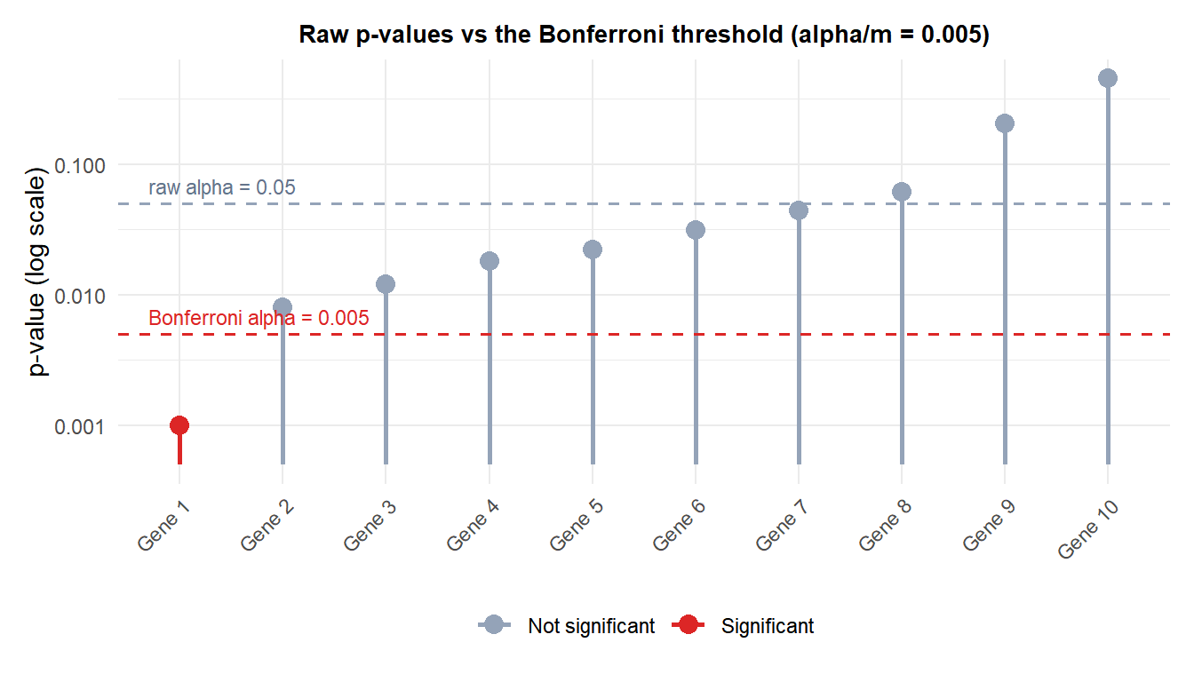
A researcher compares expression levels for 10 genes between two conditions, running 10 separate t-tests and getting these raw p-values:
\[0.001,\ 0.008,\ 0.012,\ 0.018,\ 0.022,\ 0.031,\ 0.044,\ 0.061,\ 0.204,\ 0.450\]
At the raw threshold \(\alpha=0.05\), 7 of the 10 genes look “significant” (all except the last three: 0.061, 0.204, 0.450). But with \(m=10\) tests, the Bonferroni-corrected threshold is \(\alpha/m = 0.05/10 = 0.005\).
| Raw p-value | Bonferroni-adjusted p-value (\(p \times 10\), capped at 1) | Significant at adjusted \(\alpha=0.05\)? |
|---|---|---|
| 0.001 | 0.010 | Yes |
| 0.008 | 0.080 | No |
| 0.012 | 0.120 | No |
| 0.018 | 0.180 | No |
| 0.022 | 0.220 | No |
| 0.031 | 0.310 | No |
| 0.044 | 0.440 | No |
| 0.061 | 0.610 | No |
| 0.204 | 1.000 | No |
| 0.450 | 1.000 | No |
Only 1 of the 10 genes survives the correction. What looked like 7 “hits” at the raw threshold shrinks to a single robust finding once the correction accounts for having run 10 tests. This is the entire point of the correction: most of those raw “significant” results were exactly the kind of false positives the multiple comparisons problem predicts.

Holm’s step-down method: a strictly better Bonferroni
Holm’s procedure is uniformly more powerful than plain Bonferroni while still controlling the familywise error rate exactly at \(\alpha\), so there is rarely a good reason to prefer plain Bonferroni over it in practice. It works as a step-down procedure:
- Sort the p-values ascending: \(p_{(1)} \leq p_{(2)} \leq \cdots \leq p_{(m)}\).
- Compare the \(i\)-th smallest p-value to \(\alpha/(m-i+1)\).
- Starting from \(i=1\), reject each hypothesis as long as its p-value is below its threshold. Stop at the first failure, and do not reject that hypothesis or any with a larger p-value.
For the gene expression example, Holm’s procedure also only rejects the smallest p-value. The smallest, 0.001, is compared to \(\alpha/(10-1+1) = 0.05/10 = 0.005\) and passes. The second-smallest, 0.008, is compared to \(\alpha/(10-2+1) = 0.05/9 \approx 0.0056\) and fails, since \(0.008 > 0.0056\). The step-down procedure stops there, so the final conclusion is the same as plain Bonferroni in this particular example: only 1 of the 10 genes is significant. But this agreement is a coincidence of this dataset, not a general rule: Holm’s method is never less powerful than Bonferroni, and often is more powerful, so it should be the practical default whenever a simple familywise-error correction is wanted.
The reason Holm can only do better than Bonferroni is in the thresholds themselves. Plain Bonferroni compares every single p-value to the same strict \(\alpha/m\). Holm’s step-down thresholds start at that same strictest value for the smallest p-value, but loosen at each subsequent step, from \(\alpha/m\) up toward \(\alpha/(m-1)\), \(\alpha/(m-2)\), and so on, since fewer hypotheses remain “in play” once earlier ones have already been rejected. This means Holm’s procedure can never reject fewer hypotheses than Bonferroni, and often rejects strictly more, all while providing the exact same familywise error rate guarantee.
⚠️ Bonferroni is conservative, and controls a different error rate than you might expect
Bonferroni (and Holm) control the familywise error rate: the probability of any false positive at all among all \(m\) tests. That is a strict standard, appropriate when even a single false positive would be costly, for example approving a single ineffective drug variant, or wrongly flagging a single employee for fraud. But it becomes extremely conservative as \(m\) grows large. In exploratory settings with hundreds or thousands of tests, like screening thousands of genes or hundreds of website A/B test metrics, Bonferroni will bury almost every real, true effect under an overwhelming number of comparisons. For those large-scale exploratory settings, control the false discovery rate instead (the expected proportion of false positives among the results you call significant), using the Benjamini-Hochberg procedure.
Benjamini-Hochberg (FDR): a less conservative alternative for large-scale testing
The false discovery rate (FDR) framing asks a different question than the familywise error rate. FWER asks “what is the chance of any false positive at all?”. FDR instead asks “of the results I flag as significant, what fraction are expected to be false?”. Tolerating a small, controlled fraction of false positives among your discoveries, instead of guarding against any single one, is far less conservative and much more powerful for detecting real effects when \(m\) is large.
The Benjamini-Hochberg (BH) procedure:
- Sort the p-values ascending: \(p_{(1)} \leq p_{(2)} \leq \cdots \leq p_{(m)}\).
- Find the largest \(i\) such that \(p_{(i)} \leq \frac{i}{m}\alpha\).
- Reject all hypotheses up to and including that \(i\)-th one.
Unlike Bonferroni and Holm, whose thresholds get stricter (or stay flat) as \(m\) grows, the BH thresholds \(\frac{i}{m}\alpha\) increase linearly with rank \(i\). The largest p-value is allowed all the way up to \(\alpha\) itself, while the smallest is held to the strictest threshold \(\alpha/m\). This sliding scale is what makes BH much less conservative than a flat \(\alpha/m\) cutoff applied to every test.
Applying BH to the same 10 gene p-values, with \(\alpha=0.05\) and \(m=10\):
| Rank \(i\) | p-value \(p_{(i)}\) | Threshold \(\frac{i}{10}\alpha\) | Below threshold? |
|---|---|---|---|
| 1 | 0.001 | 0.005 | Yes |
| 2 | 0.008 | 0.010 | Yes |
| 3 | 0.012 | 0.015 | Yes |
| 4 | 0.018 | 0.020 | Yes |
| 5 | 0.022 | 0.025 | Yes |
| 6 | 0.031 | 0.030 | No |
| 7 | 0.044 | 0.035 | No |
| 8 | 0.061 | 0.040 | No |
| 9 | 0.204 | 0.045 | No |
| 10 | 0.450 | 0.050 | No |
The largest rank still below its own threshold is \(i=5\), so the procedure rejects the first 5 hypotheses (p-values 0.001, 0.008, 0.012, 0.018 and 0.022), compared to just 1 for Bonferroni or Holm. Note that rank 6 (p = 0.031) fails its threshold even though rank 5 passed: BH looks for the largest qualifying rank across the whole sorted list, it does not simply stop at the first failure the way Holm’s step-down procedure does.
Same data, three very different numbers of “significant” results: 7 at the raw threshold, 1 with Bonferroni or Holm, and 5 with BH. This concretely shows why picking the right correction for your actual research question, FWER versus FDR, matters just as much as correcting for multiple comparisons at all.
Running the correction in R
The same ten p-values from above, adjusted all three ways with a single built-in function:
pvals <- c(0.001, 0.008, 0.012, 0.018, 0.022, 0.031, 0.044, 0.061, 0.204, 0.450)

p.adjust(pvals, method = "bonferroni")   # simplest, most conservative
p.adjust(pvals, method = "holm")         # uniformly more powerful than Bonferroni
p.adjust(pvals, method = "BH")           # Benjamini-Hochberg, controls FDR instead of FWER

# Decision at alpha = 0.05
data.frame(p = pvals,
           bonferroni = p.adjust(pvals, method = "bonferroni") < 0.05,
           holm       = p.adjust(pvals, method = "holm")       < 0.05,
           BH         = p.adjust(pvals, method = "BH")         < 0.05)
💡 Which correction to use
Use Bonferroni only when you need the simplest possible explanation and have very few tests (a handful), or need a correction that is guaranteed valid even under unknown or arbitrary dependence between tests. In almost every other case, prefer Holm’s method over plain Bonferroni: it is strictly more powerful, gives the same guarantee, and is just as simple to apply. For large-scale exploratory screening, many dozens or hundreds of tests, where you can tolerate a controlled small fraction of false positives among your discoveries rather than guarding against any single one, use Benjamini-Hochberg instead. The right choice depends on whether a single false positive would be costly (use FWER: Bonferroni or Holm) or whether you mainly want to control the overall proportion of false leads among your findings (use FDR: Benjamini-Hochberg).

