Quantile regression
Ordinary least squares models the conditional MEAN of \(y\) given \(x\): one line, one number, one slope. Quantile regression instead models a conditional QUANTILE, the median, the 10th percentile, the 90th percentile, or any percentile you choose. That distinction matters whenever a predictor changes not just the average outcome but the spread or shape of the whole distribution, exactly the kind of pattern a single mean line hides completely.
Modeling the mean is not the whole story
A single OLS fit answers one question: how does the average of \(y\) shift as \(x\) changes? It says nothing about whether the variability of \(y\) also changes with \(x\). When the data is heteroscedastic, the spread of \(y\) around its center genuinely widens or narrows across the range of \(x\), and when the outcome is skewed, the mean itself can be a misleading summary (see why the average lies). Quantile regression fits a separate line for each quantile of interest, so it can show that the relationship between \(x\) and \(y\) is not just a shift in level, it can be a change in shape.
The check function (pinball loss)
Quantile regression for quantile \(\tau \in (0,1)\) finds the coefficients that minimize the check function, also called the pinball loss, applied to the residuals \(u = y - \hat y\):
\[\rho_\tau(u) = u\left(\tau - \mathbb{1}(u < 0)\right) = \begin{cases} \tau \cdot u & u \geq 0 \\ (\tau - 1) \cdot u & u < 0 \end{cases}\]
This loss weights positive and negative residuals asymmetrically whenever \(\tau \neq 0.5\): for \(\tau = 0.9\), underpredicting (a positive residual) costs \(0.9\) per unit while overpredicting costs only \(0.1\) per unit, so the fitted line is pulled up until exactly 90% of points fall below it. At \(\tau = 0.5\) the loss becomes symmetric and proportional to \(|u|\), which is ordinary least absolute deviations (LAD) regression, the median regression case. Ordinary least squares is a different loss altogether, squared error, \(u^2\), which targets the conditional mean rather than any particular quantile. OLS is not a special case of the check function; it is a separate loss function that happens to answer a related but distinct question.
Worked example: Engel’s food expenditure data
A real 19th-century household budget dataset, still standard for teaching this method, makes the widening spread concrete.
The classic dataset for this method is the one Koenker and Bassett used in their original 1978 quantile regression paper: 235 Belgian working-class household budgets compiled by the statistician Ernst Engel in 1857, relating household income to food expenditure (both in Belgian francs). It ships with R’s quantreg package as engel. Note this is Ernst Engel the 19th-century statistician, not Friedrich Engels the co-author of the Communist Manifesto, an easy pair to mix up.
Income in the sample ranges from 377 to 4,958 francs. The OLS fit gives:
\[\widehat{\text{foodexp}} = 147.48 + 0.485 \cdot \text{income}, \quad R^2 = 0.830\]
Fitting three quantile regressions at \(\tau = 0.1, 0.5, 0.9\) gives three different lines, not three parallel shifts of the same line:
| Quantile | Intercept | Slope |
|---|---|---|
| \(\tau = 0.1\) | 110.14 | 0.402 |
| \(\tau = 0.5\) (median) | 81.48 | 0.560 |
| \(\tau = 0.9\) | 67.35 | 0.686 |
The slope itself climbs from 0.402 at the 10th percentile to 0.686 at the 90th, a pattern invisible to the single OLS slope of 0.485.

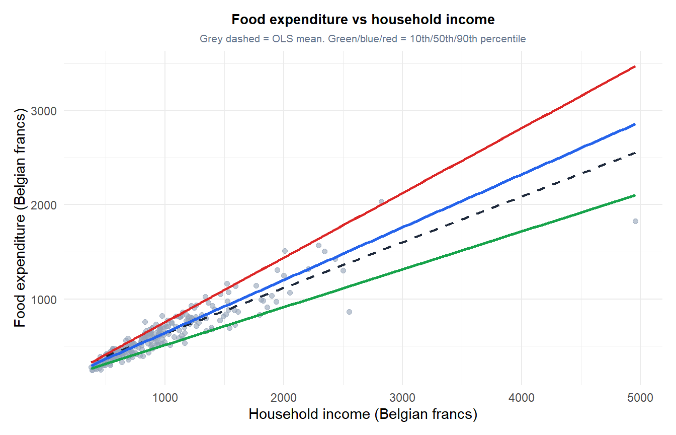
What changes across the quantiles
Plugging the poorest and richest households in the sample into each fitted line:
| Income | OLS mean | \(\tau=0.1\) | \(\tau=0.5\) | \(\tau=0.9\) | Gap (\(\tau=0.9\) minus \(\tau=0.1\)) |
|---|---|---|---|---|---|
| 377 (minimum) | 330 | 262 | 293 | 326 | 64.5 |
| 4,958 (maximum) | 2,553 | 2,102 | 2,859 | 3,470 | 1,367.9 |
At the lowest income in the sample, the gap between the 10th and 90th percentile household is only about 65 francs, poor households spend on food in a fairly narrow, disciplined band. At the highest income, that gap balloons to almost 1,368 francs, more than 20 times wider, rich households show far more discretion in how much of their income goes to food. The single OLS line, with its one slope of 0.485, reports only the average trend and hides this widening entirely.
This dataset also happens to be the one that established Engel’s law: food’s share of the budget falls as income rises. The OLS fit predicts food spending equal to about 87.6% of income at the poorest end of the sample and only about 51.5% at the richest, even though the absolute amount spent on food keeps rising throughout.
Not the same as inspecting residual spread
The rising slope in the table above is easy to misread as just a wider scatter of residuals around one mean line, but that is not what is actually happening.
⚠️ Each quantile line is its own separate fit, not a shifted copy of the OLS line
It is tempting to think quantile regression is just “fit OLS, then look at how wide the residuals are.” It is not. Each \(\tau\) line above is fit independently and can have its own slope, as the table shows: the slope genuinely increases from 0.402 to 0.686 across the three quantiles. A model that only shifted a single OLS line up or down (constant slope, different intercepts) would completely miss this: the relationship between income and food spending is not just shifting, it is changing shape across the distribution, and only fitting a separate line per quantile reveals that.
When to reach for quantile regression
- Heteroscedastic data, where the spread of \(y\) visibly changes with \(x\), exactly the pattern regression diagnostics normally flags as a violation to fix or at least tolerate in an OLS model. In quantile regression, that same widening spread is not a nuisance to correct, it is the object of interest.
- Skewed outcomes, where the mean is pulled away from what a “typical” observation looks like, and where the median or another quantile is a more informative summary (see why the average lies).
- Questions about the tails, not just the center: a policy question like “what income threshold would move the poorest 10% of a target group” needs the 10th percentile’s own model, not an adjustment to the mean.
- Robustness to outliers in \(y\): because it is built on absolute rather than squared deviations from the fitted quantile, an extreme \(y\) value has bounded influence, unlike its unbounded influence on an OLS mean.
Running it in R
quantreg::rq() mirrors lm()’s syntax closely, with the quantile of interest set through the tau argument:
library(quantreg)
data(engel)

# Median regression (tau = 0.5)
rq(foodexp ~ income, data = engel, tau = 0.5)

# Several quantiles at once
rq(foodexp ~ income, data = engel, tau = c(0.1, 0.5, 0.9))

# Compare against the conditional mean
lm(foodexp ~ income, data = engel)
💡 Quantile regression coefficients are interpreted per quantile
A coefficient from rq(y ~ x, tau = 0.9) means: holding other predictors fixed, a one-unit increase in \(x\) is associated with a change of that size in the 90th percentile of \(y\), not in its mean. Standard errors for quantile regression are typically obtained by bootstrap (rq’s default) rather than the closed-form formulas used for OLS, since the check function is not differentiable at zero.

