Dickey-Fuller test
The general stationarity post introduces the unit root and mentions the ADF and KPSS tests briefly. This post goes deep into a single test: how the (Augmented) Dickey-Fuller regression is actually built, why its critical values are not the ones in a normal t-table, and a full worked example computed by hand from real R output.
The Dickey-Fuller regression
Start from the simple AR(1) process:
\[y_t = \phi y_{t-1} + \varepsilon_t\]
Subtracting \(y_{t-1}\) from both sides gives an algebraically equivalent regression form:
\[y_t - y_{t-1} = (\phi - 1) y_{t-1} + \varepsilon_t \quad \implies \quad \Delta y_t = \gamma y_{t-1} + \varepsilon_t, \qquad \gamma = \phi - 1\]
This rewriting turns the hard question “is \(\phi = 1\)?” into an easy one: “is \(\gamma = 0\)?”, something an ordinary regression coefficient can answer directly.
\[H_0: \gamma = 0 \ \ (\phi = 1,\ \text{unit root, non-stationary})\] \[H_1: \gamma < 0 \ \ (\phi < 1,\ \text{stationary})\]
In practice, three specifications are used, matching the type= argument of urca::ur.df():
none: no constant, no trend. \(\Delta y_t = \gamma y_{t-1} + \varepsilon_t\).drift: constant only, no trend. \(\Delta y_t = \alpha + \gamma y_{t-1} + \varepsilon_t\).trend: constant plus a linear trend. \(\Delta y_t = \alpha + \beta t + \gamma y_{t-1} + \varepsilon_t\).
The drift specification is the most common default for series without an obvious deterministic trend, and it is the one used in the worked example below. Picking the wrong specification costs statistical power in both directions: including a trend term when the series has none wastes degrees of freedom and makes the test less likely to reject a false unit root, while omitting a trend that is genuinely present can make a trending non-stationary series look deceptively close to stationary.
\[\Delta y_t = \alpha + \gamma y_{t-1} + \varepsilon_t \qquad H_0: \gamma = 0 \quad \text{vs} \quad H_1: \gamma < 0\]
Each specification has its own table of critical values, since adding a constant or a trend shifts the reference distribution of \(\tau\). MacKinnon’s naming convention labels these \(\tau_1\) (none), \(\tau_2\) (drift) and \(\tau_3\) (trend); summary(ur.df(...)) prints the matching one automatically depending on type=.
Why not a normal t-table?
This is the point most easily missed: under \(H_0\), \(y_{t-1}\) is itself non-stationary (it is a unit root process), so the t-statistic on \(\gamma\), usually denoted \(\tau\) (tau), does not follow a standard Student-t distribution, not even asymptotically as the sample size grows.
Intuitively, under a unit root the regressor \(y_{t-1}\) keeps drifting further from its starting point as \(t\) grows, so it does not settle down into the fixed, well-behaved distribution that ordinary least-squares theory relies on. The sampling distribution of \(\tau\) ends up skewed to the left and shifted away from the familiar bell shape, which is why relying on standard t critical values would make the test reject far too rarely.
Dickey and Fuller derived the correct reference distribution by simulation and tabulated critical values for it. MacKinnon later made these usable for any sample size through response-surface regressions, which is what packages like urca use internally to print critical values or p-values. This is why \(\tau\) must always be compared against special Dickey-Fuller (or MacKinnon) critical values, never against qt() or a printed t-table.
Augmenting for autocorrelation (the “A” in ADF)
The regression above assumes the errors \(\varepsilon_t\) are white noise. If \(y_t\) has higher-order autocorrelation, the residuals will not be white noise and the test becomes unreliable. The fix is to add lagged difference terms until the residuals are whitened:
\[\Delta y_t = \alpha + \gamma y_{t-1} + \sum_{j=1}^p \delta_j \Delta y_{t-j} + \varepsilon_t\]
The number of lags \(p\) is typically chosen by AIC or BIC, or by a sequential procedure: start with a generous number of lags and drop the least significant one until the last included lag is significant. Adding lags only controls for autocorrelation; the hypothesis test itself is still on \(\gamma\), unchanged.
Too few lags leave autocorrelation in the residuals and distort the size of the test, making it reject too often. Too many lags waste degrees of freedom and reduce power, making it harder to reject a false unit root. In practice this trade-off is exactly why urca::ur.df() exposes lags as an argument rather than hardcoding a single choice.
A common rule of thumb for the starting number of lags, due to Schwert, is \(p_{max} = \lfloor 12 (T/100)^{1/4} \rfloor\), after which AIC, BIC or the sequential t-test procedure trims it down. For the short series used in the worked example below, \(T=60\), that upper bound is already small enough that testing with lags = 0 is a reasonable simplification for illustration.
A worked example, by hand
Running the test side by side on a genuinely stationary series and a genuinely non-stationary one shows exactly what the test statistic and \(p\)-value look like in each case.
Simulate two series of length \(T=60\): a stationary AR(1) process with \(\phi=0.6\), and a pure random walk.
set.seed(1)
T <- 60
eps  <- rnorm(T)
y_ar <- numeric(T)
for (t in 2:T) y_ar[t] <- 0.6 * y_ar[t-1] + eps[t]
eps2 <- rnorm(T)
y_rw <- cumsum(eps2)
Both are tested with the drift specification and no augmentation lags (urca::ur.df(y, type = "drift", lags = 0)).
For y_ar (the stationary AR(1) series):
\[\widehat{\Delta y_t} = 0.165 - 0.550\, y_{t-1}\]
\(SE(\hat\gamma) = 0.118\), so \(\tau = -0.550/0.118 = -4.655\), with residual \(df = 57\).
For y_rw (the random walk):
\[\widehat{\Delta y_t} = 0.417 - 0.083\, y_{t-1}\]
\(SE(\hat\gamma) = 0.0547\), so \(\tau = -0.083/0.0547 = -1.509\), with residual \(df = 57\).
MacKinnon critical values for the drift specification (\(\tau_2\)): 1% = \(-3.51\), 5% = \(-2.89\), 10% = \(-2.58\).
Decision for y_ar: \(\tau = -4.655 < -3.51\), so \(H_0\) is rejected at the 1% level. Strong evidence of stationarity, correctly matching how the series was simulated: an AR(1) with \(|\phi| < 1\).
Decision for y_rw: \(\tau = -1.509\), which is greater than even the 10% critical value (\(-2.58\)), i.e. less negative, inside the non-rejection region. \(H_0\) is not rejected. No evidence against the unit root, correctly matching how the series was simulated: a pure random walk.

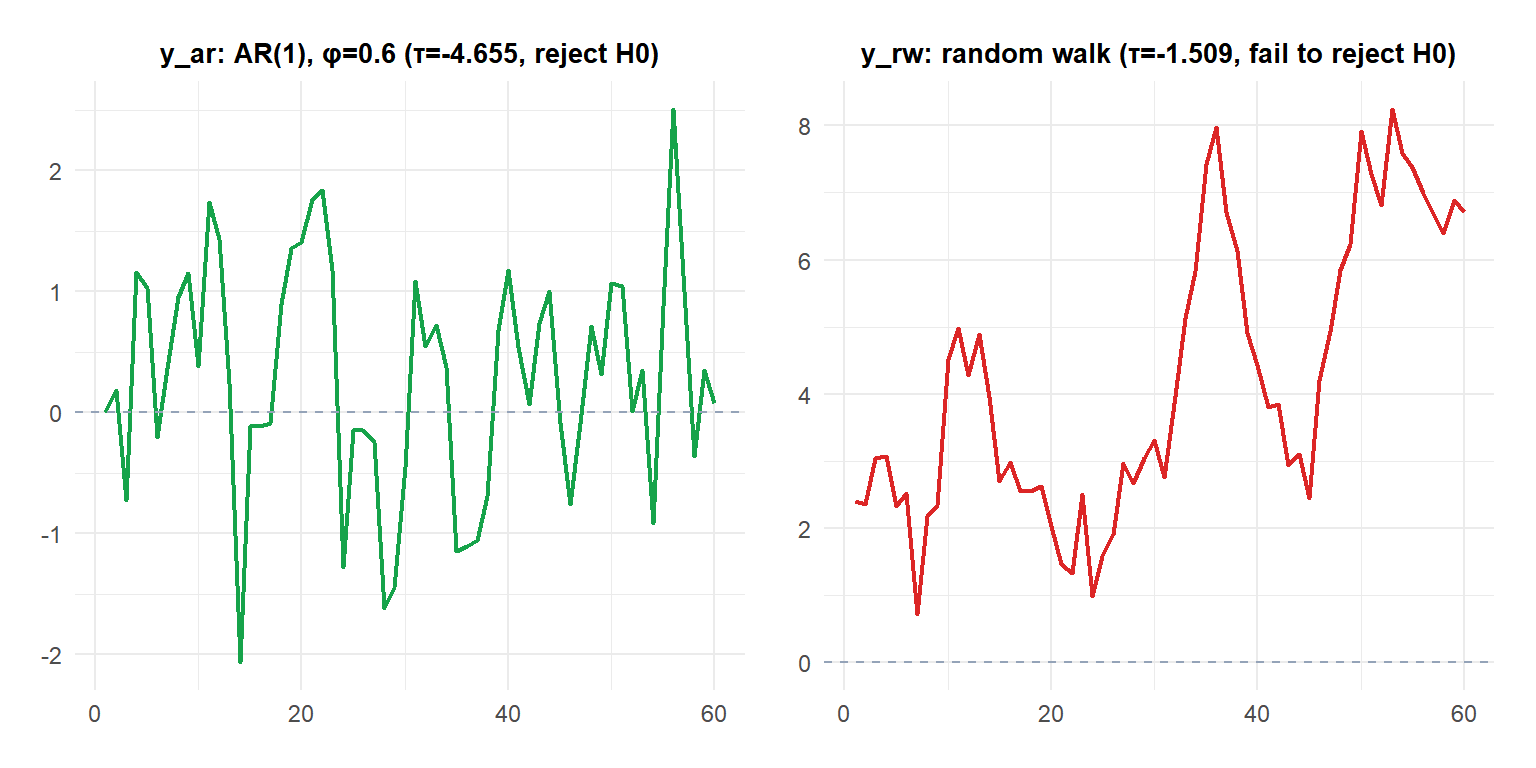
The stationary series (green) hovers around a constant mean and keeps crossing the zero line. The random walk (red) wanders away from zero and never reliably comes back, exactly the visual signature the ADF test picks up numerically.
Notice the direction of the two standard errors relative to \(\hat\gamma\): for y_ar, \(SE(\hat\gamma) = 0.118\) is small relative to the coefficient, so the coefficient is estimated precisely enough to be distinguishable from zero. For y_rw, \(SE(\hat\gamma) = 0.0547\) is small in absolute terms too, but the coefficient itself, \(-0.083\), is close enough to zero that \(\tau\) still lands well inside the non-rejection region.
⚠️ tseries::adf.test() is not the same regression: check what it actually fits
R’s tseries::adf.test() by default fits a different specification than the drift-only one above: it includes both a constant and a linear trend term, and it automatically picks the augmentation lag order via a rule of thumb, \(p = \lfloor (n-1)^{1/3} \rfloor\). The worked example above instead used urca::ur.df(type = "drift", lags = 0): constant only, no augmentation.
Because the specification differs, adf.test()’s printed statistic and p-value will generally not match the drift, no-augmentation numbers computed above. Both are valid ADF tests, they just answer a subtly different question: whether there is a deterministic trend to control for, and how many autocorrelation lags are needed to whiten the residuals. Always check which specification a function is using (type= in urca::ur.df(), or the documentation for whatever package you use) before comparing results across tools or papers.
Choosing between ADF, KPSS and Phillips-Perron
ADF tests \(H_0\) = unit root, while KPSS tests the opposite, \(H_0\) = stationary, so a robust conclusion needs both tests to agree rather than relying on either one alone. The general stationarity post covers KPSS and Phillips-Perron in more depth; here is just a compact reminder.
| Test | \(H_0\) | Rejecting \(H_0\) means |
|---|---|---|
| ADF | Unit root (non-stationary) | Evidence of stationarity |
| KPSS | Stationary | Evidence of a unit root |
| Phillips-Perron | Unit root (non-stationary) | Evidence of stationarity (robust to heteroscedasticity) |
Running the test in R
summary() on a ur.df() object prints the fitted regression coefficients, the test statistic (labeled tau2 for the drift specification), and a small table of critical values at the 1%, 5% and 10% levels, the same numbers used in the worked example above. Reading that table directly, rather than a p-value alone, is good practice: it shows exactly how close the decision was to the next significance level.
library(urca)

set.seed(1)
T <- 60
eps  <- rnorm(T)
y_ar <- numeric(T)
for (t in 2:T) y_ar[t] <- 0.6 * y_ar[t-1] + eps[t]
eps2 <- rnorm(T)
y_rw <- cumsum(eps2)

# Transparent regression form, exactly matching the by-hand example
summary(ur.df(y_ar, type = "drift", lags = 0))
summary(ur.df(y_rw, type = "drift", lags = 0))

# Quick, commonly used alternative (different default specification, see warning above)
library(tseries)
adf.test(y_ar)
adf.test(y_rw)

# Automatic order-of-differencing helper
library(forecast)
ndiffs(y_rw)
ndiffs() runs exactly this kind of ADF-based search internally (KPSS is also an option via its test= argument) and returns the minimum number of regular differences it estimates are needed, which is a convenient shortcut once you already understand what the underlying regression is doing.
💡 Always difference and retest
If the ADF test fails to reject the unit root, the standard remedy is to first-difference the series and run the ADF test again on \(\Delta y_t\). Repeat until the test rejects. Most economic and financial series are integrated of order 1, \(I(1)\): one difference is enough. forecast::ndiffs() automates this search. Over-differencing, going further than needed, introduces unnecessary noise and should be avoided: always confirm the minimum \(d\) that achieves stationarity rather than differencing repeatedly “to be safe”.

