Granger causality

Granger causality asks a purely predictive question: does the past of one time series help predict another, beyond what that series’ own past already tells you? This post builds on the brief mention in the VAR model post, walking through the restricted-vs-unrestricted F-test by hand and showing exactly why the test can detect a real, asymmetric predictive relationship.

Restricted vs unrestricted regression

To test whether \(x\) Granger-causes \(y\) at lag \(p\), compare two nested regressions of \(y\) on its own past:

\[H_0: \gamma_1 = \gamma_2 = \cdots = \gamma_p = 0 \quad (x \text{ does not Granger-cause } y)\]

Test \(H_0\) with an F-test comparing how much the residual sum of squares drops when the \(x\) lags are added:

\[F = \frac{(RSS_r - RSS_u)/q}{RSS_u/(n-k)}\]

where \(q\) is the number of restrictions (the \(p\) dropped \(x\) lags) and \(k\) is the number of parameters in the unrestricted model.

Worked example: does x really drive y?

Building the asymmetry directly into the simulation, \(x\) drives \(y\) but never the reverse, makes it possible to check that testing both directions actually recovers that one-way relationship.

Two simulated series with a known, asymmetric relationship

Simulate two series where \(x\) truly drives \(y\) with a one-period lag, and \(y\) does NOT drive \(x\), so the test should correctly detect the asymmetry:

set.seed(1)
T <- 100
x <- numeric(T); y <- numeric(T)
for (t in 2:T) x[t] <- 0.5 * x[t-1] + rnorm(1)
for (t in 3:T) y[t] <- 0.3 * y[t-1] + 0.5 * x[t-1] + rnorm(1)

Testing lag 1 on observations \(t=3,\ldots,100\) (\(n=98\)):

Restricted model: \(\hat y_t = 0.094 + 0.339\, y_{t-1}\), \(RSS_r = 107.80\), residual df \(= 96\).

Unrestricted model: \(\hat y_t = -0.019 + 0.303\, y_{t-1} + 0.446\, x_{t-1}\), \(RSS_u = 89.47\), residual df \(= 95\).

\[F = \frac{(107.80 - 89.47)/1}{89.47/95} = \frac{18.33}{0.9418} = 19.46\]

\(df = (1, 95)\), \(p = 2.71 \times 10^{-5}\). Decision: reject \(H_0\), \(x\) Granger-causes \(y\).

Now test the REVERSE direction (does \(y\) Granger-cause \(x\)?), same data, same lag: \(F = 1.17\), \(df = (1, 95)\), \(p = 0.282\). Decision: fail to reject \(H_0\), no evidence that \(y\) Granger-causes \(x\), correctly matching the true data-generating process (only \(x\) drove \(y\), never the other way around).

lmtest::grangertest() run on the same data reproduces this closely (forward: \(F \approx 19.67\), \(p \approx 2.45 \times 10^{-5}\); reverse: \(F = 1.17\), \(p = 0.282\)); the tiny numeric difference from the by-hand numbers is only due to how the helper function internally aligns the lagged sample, not a real disagreement.

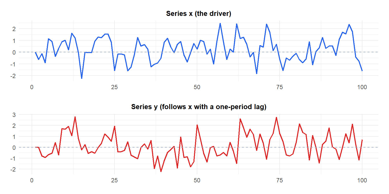
Visually, spikes in \(x\) tend to be echoed in \(y\) one step later, exactly the lagged dependency the F-test picks up.

Extending to a full VAR framework

In practice, Granger causality is usually tested inside a fitted VAR model with vars::causality(), which already covers VAR estimation, lag selection by AIC/BIC, impulse response functions, and forecast error variance decomposition. The two-series, single-lag example above is the simplest case of the exact same underlying F-test logic, generalized in a VAR to any number of variables and lags at once.

Running the test in R

The by-hand F-test above can be reproduced directly, and cross-checked, with lmtest::grangertest():

set.seed(1)
T <- 100
x <- numeric(T); y <- numeric(T)
for (t in 2:T) x[t] <- 0.5 * x[t-1] + rnorm(1)
for (t in 3:T) y[t] <- 0.3 * y[t-1] + 0.5 * x[t-1] + rnorm(1)

library(lmtest)
grangertest(y ~ x, order = 1)   # does x Granger-cause y?
grangertest(x ~ y, order = 1)   # does y Granger-cause x?

# Inside a fitted VAR model
library(vars)
fit <- VAR(cbind(x, y), p = 1, type = "const")
causality(fit, cause = "x")