Method of moments estimation
The method of moments estimates a distribution’s parameters by setting its theoretical moments, the mean, the variance, and so on, equal to the sample’s observed moments, then solving for the parameters. It is older and simpler than maximum likelihood estimation: it usually needs only algebra, no calculus and no numerical optimization.
The general recipe
For a distribution with \(k\) unknown parameters, equate the first \(k\) theoretical moments to the corresponding sample moments, and solve the resulting system of \(k\) equations for the \(k\) parameters:
\[E[X^j] = \frac{1}{n}\sum_{i=1}^n x_i^j, \qquad j = 1, \ldots, k\]
The left side is a known formula in terms of the parameters, since it comes from the distribution’s own definition. The right side is just a number, computed directly from the sample. Each equation pins down one more parameter, so a distribution with 2 unknown parameters needs the first 2 moments; one with 1 unknown parameter needs only the mean.
Worked example: fitting a Gamma distribution
The Gamma distribution has two parameters, so it needs the first two moments: the mean and the variance.
A simulated sample of \(n=200\) observations from a Gamma distribution with true shape \(k=4\) and true rate \(=0.5\) (mean \(8\), variance \(16\)). Using the Gamma distribution’s own moment formulas, \(E[X] = k\theta\) and \(\text{Var}(X) = k\theta^2\) (with scale \(\theta = 1/\text{rate}\)), solving for the two parameters from the sample mean \(\bar{x}\) and sample variance \(s^2\) gives:
\[\hat{k}_{MoM} = \frac{\bar{x}^2}{s^2}, \qquad \hat{\theta}_{MoM} = \frac{s^2}{\bar{x}}\]
On this sample, \(\bar{x} = 7.691\) and \(s^2 = 14.162\), so:
| Parameter | Method of moments | Maximum likelihood | True value |
|---|---|---|---|
| Shape (\(k\)) | 4.176 | 4.010 | 4 |
| Rate | 0.543 | 0.521 | 0.5 |
Both methods land close to the truth and close to each other, the method of moments estimate is not identical to the maximum likelihood estimate, the two optimize different criteria, but on a reasonably sized sample from a well-behaved distribution they typically agree to within a few percent.

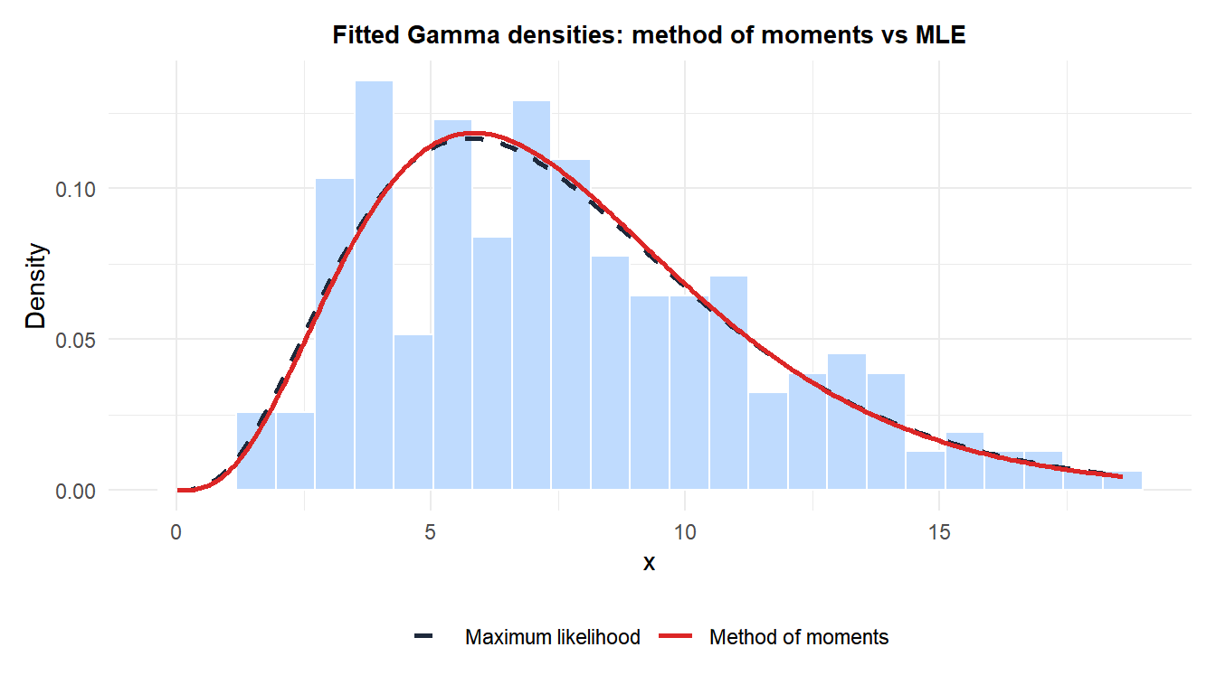
The two fitted curves nearly overlap. For a well-specified, reasonably large sample, the choice between the two methods rarely changes the practical conclusion, the difference shows up in efficiency (how much the estimates bounce around from sample to sample), not in a visibly different fit to this particular dataset.
Where the method of moments falls short
Equating sample and theoretical moments is simple, but the simplicity has real costs.
⚠️ Method of moments estimators are not always valid, and rarely as efficient as MLE
Because the method of moments solves whatever algebra the moment equations produce, it can occasionally return a nonsensical estimate, for example a negative implied variance parameter from a small or unusual sample, something a properly constrained MLE fit normally avoids. It is also generally less efficient than MLE: for the same sample, the method of moments estimator typically has a larger sampling variance, meaning it bounces around more from sample to sample. In practice, method of moments estimates are often used mainly as good starting values for an iterative MLE optimization, rather than as the final reported estimate.
Running it in R
The method of moments needs nothing beyond mean() and var(); maximum likelihood needs an optimizer, usually hidden inside a fitting function:
x <- rgamma(200, shape = 4, rate = 0.5)

# Method of moments, closed-form algebra
xbar <- mean(x)
s2   <- var(x)
k_hat_mom     <- xbar^2 / s2
theta_hat_mom <- s2 / xbar

# Maximum likelihood, via numerical optimization under the hood
library(MASS)
fit_mle <- fitdistr(x, "gamma")
fit_mle$estimate
💡 Why MLE became the default anyway
If method of moments is simpler, why is MLE the one built into glm(), fitdistr(), and almost every other modern fitting function? Because MLE’s efficiency advantage, achieving the lowest possible sampling variance among consistent estimators as the sample grows, generally outweighs the convenience of closed-form algebra, now that computers make numerical optimization essentially free. The method of moments still earns its keep for quick back-of-the-envelope estimates, for distributions where MLE has no closed form and needs a sensible starting value, and for teaching the core idea, matching the data’s own moments, before introducing likelihood.

