Bartlett's test
Bartlett’s test checks whether two or more groups have equal population variances, exactly the same question as Levene’s test, but it assumes the data are normally distributed within each group, unlike Levene’s test which makes no such assumption. When normality genuinely holds, Bartlett is more powerful; when it doesn’t, Bartlett becomes unreliable, prone to false positives. It also generalizes the two-group F-test to any number of groups.
Hypotheses
\[H_0: \sigma_1^2 = \sigma_2^2 = \cdots = \sigma_k^2\]
\[H_1: \text{at least one } \sigma_i^2 \text{ differs}\]
Same hypotheses as Levene’s test, only the assumptions and the test statistic differ.
Bartlett’s test statistic
The statistic compares each group’s own variance against the pooled variance across all groups, weighted by degrees of freedom:
\[B = \frac{(N-k)\ln(S_p^2) - \sum_{i=1}^k (n_i-1)\ln(S_i^2)}{C}\]
where the pooled variance is \(S_p^2 = \frac{\sum_i (n_i-1)S_i^2}{N-k}\), and \(C = 1 + \frac{1}{3(k-1)}\left(\sum_i \frac{1}{n_i-1} - \frac{1}{N-k}\right)\) is a small-sample correction factor. Under \(H_0\), \(B \sim \chi^2(k-1)\) approximately.
Worked example: same data as the Levene’s test post
Reusing the exact same three machines makes it possible to compare Bartlett’s result directly against Levene’s on identical data.
Three machines each produce 5 units; quality engineers measure a dimension (mm) to check whether the machines are equally consistent:
- Machine A: 23, 25, 24, 26, 22 (\(s_A^2 = 2.5\))
- Machine B: 20, 30, 15, 35, 25 (\(s_B^2 = 62.5\))
- Machine C: 24, 24, 25, 23, 24 (\(s_C^2 = 0.5\))
Pooled variance:
\[S_p^2 = \frac{4(2.5) + 4(62.5) + 4(0.5)}{12} = \frac{10+250+2}{12} = 21.833\]
Bartlett’s statistic (computed via the formula above): \(B = 17.611\), \(df = k-1 = 2\), \(p\text{-value} = 0.00015\).
Decision: reject \(H_0\) at any conventional level, the same conclusion as Levene’s test on this exact data (which gave \(W = 7.438\), \(p = 0.00792\)). Bartlett’s p-value here (0.00015) is even smaller than Levene’s (0.00792): both agree the variances differ, but Bartlett’s statistic reacts more strongly to the same data. This particular dataset happens to be close enough to normal that Bartlett behaves reliably here; the general concern, covered below, is about what happens when it isn’t.

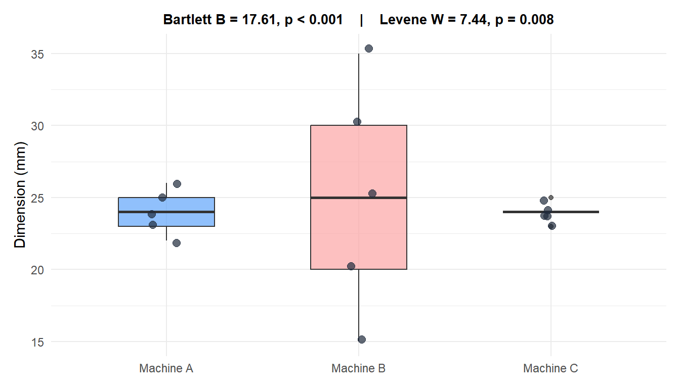
Both tests agree on this data: Machine B’s much wider spread drives a significant result either way.
Bartlett’s real weakness: sensitivity to non-normality
The machine data above happened to be well-behaved, but that is not guaranteed, and Bartlett’s test punishes departures from normality far more harshly than Levene’s does.
⚠️ Bartlett's test is extremely sensitive to non-normality
Unlike the agreement between Bartlett and Levene on the machine data above, Bartlett’s test can give a misleading significant result on non-normal data even when the true population variances are genuinely equal, purely because the data are skewed or heavy-tailed rather than because the variances actually differ. This mirrors exactly the same fragility already documented for the plain F-test, which is also a normality-dependent variance test. Levene’s test, and especially its Brown-Forsythe median-centered variant, was specifically developed to avoid this trap. Always verify normality first (Shapiro-Wilk, or a Q-Q plot) before trusting a Bartlett’s test result; if normality is in any doubt, prefer Levene’s test instead.
Bartlett vs Levene vs the F-test: choosing between them
| Test | Groups | Requires normality | Robustness to outliers |
|---|---|---|---|
| F-test | 2 only | Yes, strictly | Low |
| Bartlett’s test | 2 or more | Yes, strictly | Low |
| Levene’s test | 2 or more | No | Moderate to high |
Rule of thumb: data verified normal, use Bartlett, the most powerful choice when the assumption truly holds. Data non-normal or unverified, use Levene’s test, the safer general-purpose default.
Running the test in R
The same three machines, tested with bartlett.test() and compared side by side against leveneTest() on the identical data:
values <- c(23,25,24,26,22, 20,30,15,35,25, 24,24,25,23,24)
group  <- factor(rep(c("A","B","C"), each = 5))

bartlett.test(values ~ group)

# Compare directly against Levene's test on the same data
library(car)
leveneTest(values ~ group)
💡 Check normality before trusting Bartlett's test
Before running Bartlett’s test, check normality within each group (Shapiro-Wilk on each group separately, or Q-Q plots). If any group shows a clear departure from normality, especially skewness, switch to Levene’s test instead, and treat any Bartlett’s test result on visibly non-normal data with real skepticism: even a small p-value might just be reflecting non-normality rather than genuinely unequal variances.

