GAMLSS (Generalized Additive Models for Location, Scale and Shape)
A GAM lets the mean of the response depend smoothly on the predictors, but it still assumes a single, fixed relationship for the spread and shape of the distribution around that mean. GAMLSS (Generalized Additive Models for Location, Scale and Shape) removes that assumption: the mean, the variance, and even the skewness and kurtosis of the response can each depend on the predictors, through their own linear or smooth predictor, for almost any distribution family.
Modeling every parameter, not just the mean
A GLM or GAM links one parameter (usually the mean \(\mu\)) to the predictors. GAMLSS links up to four distribution parameters at once, each through its own linear predictor and link function:
\[g_1(\mu) = X_\mu \boldsymbol{\beta}_\mu, \quad g_2(\sigma) = X_\sigma \boldsymbol{\beta}_\sigma, \quad g_3(\nu) = X_\nu \boldsymbol{\beta}_\nu, \quad g_4(\tau) = X_\tau \boldsymbol{\beta}_\tau\]
where \(\mu\) is location (typically the mean or median), \(\sigma\) is scale (spread), and \(\nu\), \(\tau\) control skewness and kurtosis for distribution families flexible enough to have them. Each predictor matrix \(X\) can be different, so the variables driving the spread do not need to be the same as the ones driving the mean. Any of the four can also just be a constant, which is what a plain GLM does for \(\sigma\), \(\nu\) and \(\tau\).
This matters whenever the spread or shape of the response changes systematically with a predictor, a pattern an ordinary regression forces into a single, fixed residual variance and silently gets wrong.
Worked example: cost data with growing variability
A simulated dataset of \(n=150\) Gamma-distributed claim amounts, where both the mean and the relative spread increase with a predictor \(x\) (think claim size growing, and becoming proportionally less predictable, with policy value). Two models are fitted: one Gamma model with a single, constant \(\sigma\), and one GAMLSS model where \(\sigma\) is also allowed to depend on \(x\).
Fitted coefficients (log link on both \(\mu\) and \(\sigma\)):
| Parameter | Intercept | Slope on \(x\) |
|---|---|---|
| \(\mu\) (mean) | 3.505 | 0.178 |
| \(\sigma\) (scale) | -1.594 | 0.122 (\(p < 0.001\)) |
The slope on \(\sigma\) is clearly non-zero: a likelihood-ratio test comparing the constant-\(\sigma\) model against this one gives \(LRT = 24.07\) on 1 degree of freedom, \(p < 0.001\). The constant-\(\sigma\) model estimates a single spread of \(\sigma \approx 0.450\) for every value of \(x\); the GAMLSS model shows \(\sigma\) actually ranges from about \(0.26\) at \(x=2\) to \(0.61\) at \(x=9\), more than doubling.
The fit confirms it is worth the extra complexity: \(\text{AIC} = 1529.6\) for the constant-\(\sigma\) model versus \(\text{AIC} = 1507.5\) for GAMLSS, a clear improvement from letting \(\sigma\) vary.
Translating the fitted \(\mu\) and \(\sigma\) into quantiles at two values of \(x\) shows what this means in practice:
| \(x\) | Median | 10th percentile | 90th percentile | 90th \(-\) 10th |
|---|---|---|---|---|
| 2 | 46.5 | 32.6 | 63.8 | 31.3 |
| 9 | 145.4 | 56.1 | 301.0 | 244.8 |
The median rises about 3.1-fold from \(x=2\) to \(x=9\), but the 10th-to-90th-percentile spread rises about 7.8-fold over the same range. A model that only lets the mean move would predict the right center at \(x=9\) but drastically understate how wide the plausible range of outcomes really is.

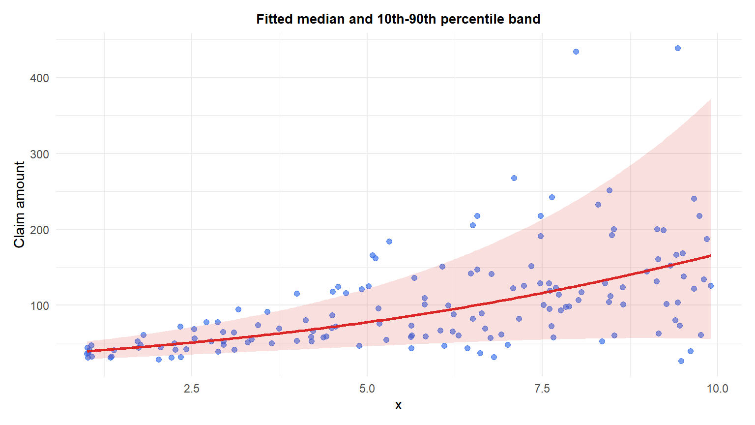
The shaded band is not a confidence interval around the mean, it is the fitted 10th-to-90th-percentile range of the response itself, and it visibly fans out as \(x\) grows, exactly the pattern a constant-\(\sigma\) model cannot represent.
GAMLSS vs quantile regression
Both approaches handle a response whose spread changes with the predictors, see quantile regression, but they work differently. Quantile regression fits each requested quantile separately with no assumed distribution, which is robust to getting the distribution family wrong but only gives you the specific quantiles you chose to fit, with no guarantee they are mutually consistent (a fitted 10th percentile line can, in principle, cross a fitted 50th percentile line). GAMLSS fits one coherent distribution per observation, so any quantile can be read off afterwards, as in the chart above, and the quantiles are guaranteed consistent by construction, but the result is only as good as the chosen distribution family.
⚠️ The distribution family is a real modeling choice
Unlike quantile regression, GAMLSS commits to a parametric family (Gamma, log-normal, a skew-t, and dozens of others are available). If the chosen family is a poor match for the data, the fitted quantiles can be systematically wrong even though the model converges without errors. Always check residual diagnostics, GAMLSS’s own wp() worm plot is the standard tool, before trusting predictions from the tails of the fitted distribution.
Running it in R
The gamlss package fits the model and lets you compare it against a constant-scale version with a likelihood-ratio test:
library(gamlss)

# Constant sigma: equivalent to an ordinary Gamma GLM
fit_const <- gamlss(y ~ x, sigma.formula = ~1, family = GA, data = df)

# GAMLSS: sigma also depends on x
fit_gamlss <- gamlss(y ~ x, sigma.formula = ~x, family = GA, data = df)

GAIC(fit_const, fit_gamlss)     # lower AIC wins
LR.test(fit_const, fit_gamlss)  # formal test of the extra sigma term

# Diagnostics
wp(fit_gamlss)                 # worm plot, checks distribution adequacy
plot(fit_gamlss)               # residual summary

# Coefficients on each parameter, and predicted quantiles
coef(fit_gamlss, what = "mu")
coef(fit_gamlss, what = "sigma")
centiles(fit_gamlss, xvar = df$x)
💡 Where GAMLSS came from
GAMLSS was introduced by Rigby and Stasinopoulos in 2005, extending earlier work on the LMS method used to build child growth reference charts, where a child’s weight or height is judged not against a single average curve but against curves for the median, spread, and skewness that all change with age. That same idea, modeling the whole shape of the distribution as it changes with a predictor rather than just its center, is what makes GAMLSS useful far beyond growth charts: insurance claims, income data, and any response where “how spread out” or “how skewed” is itself part of the story.

