R-squared and adjusted R-squared explained
R-squared is the proportion of variance in the response that a regression model explains. It is one of the first numbers anyone looks at after fitting a model, and one of the most misread: it always rises when you add a predictor, even a useless one, which is exactly what adjusted R-squared is built to correct for. This post builds on simple linear regression.
What R-squared measures
\(R^2\) compares the leftover error from the model against the total variance the model started with:
\[R^2 = 1 - \frac{SS_{res}}{SS_{tot}} = 1 - \frac{\sum_{i=1}^n (y_i-\hat y_i)^2}{\sum_{i=1}^n (y_i-\bar y)^2}\]
\(SS_{res}\) is the sum of squared residuals left over after the model, \(SS_{tot}\) is the total sum of squared deviations from the mean, the variance the model had available to explain in the first place. \(R^2\) compares the two: it is the fraction of that total variance the model accounts for.
For an in-sample fit, \(R^2\) falls between 0 (the model explains nothing beyond the mean) and 1 (the model reproduces every observed value exactly). It can go negative on new data the model was not fit to, if the model happens to predict worse than simply guessing the training mean every time.
Why R-squared always rises when you add a predictor
Ordinary least squares picks coefficients to minimize \(SS_{res}\). Adding any predictor, even one that is pure random noise unrelated to the response, gives OLS one more coefficient it is free to set to whatever value best fits the training data. The worst OLS can do with a new predictor is set its coefficient to exactly zero, reproducing the old fit. In practice, with a finite sample, some non-zero coefficient will almost always fit marginally better by chance. \(SS_{res}\) can only stay the same or shrink, so \(R^2\) can only stay the same or rise, it can never fall when a predictor is added to the same data.
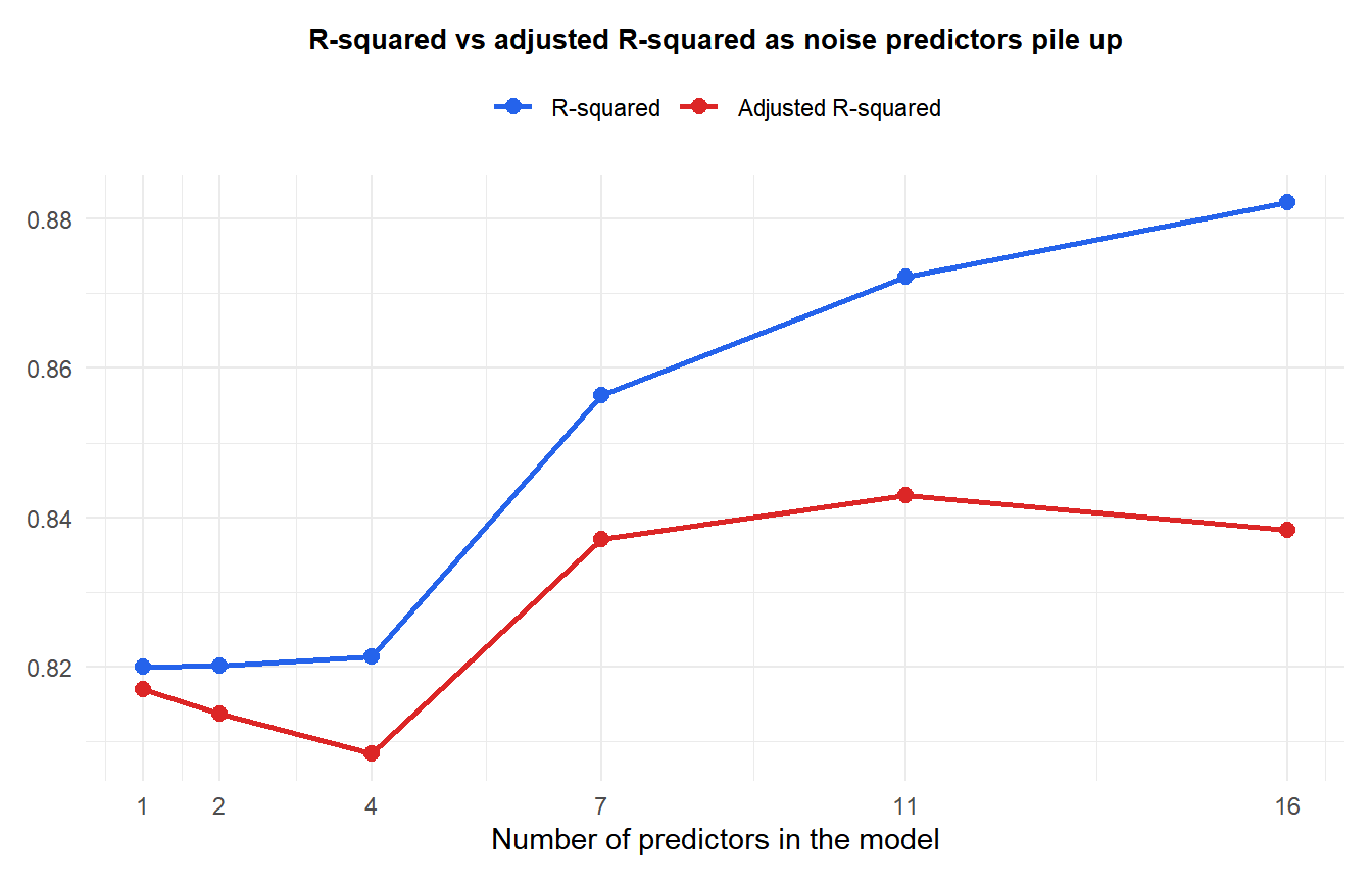
A dataset of \(n=60\) students has a real relationship between hours studied and exam score, plus natural noise: score = 40 + 5*hours_studied + noise. Starting from that single genuine predictor, random noise predictors, columns of numbers with no relationship whatsoever to the score, are added on top, one on top of the last:
| Predictors in the model | \(R^2\) | Adjusted \(R^2\) |
|---|---|---|
| 1 (just hours studied) | 0.820 | 0.817 |
| 2 (+1 noise column) | 0.820 | 0.814 |
| 4 (+3 noise columns) | 0.821 | 0.808 |
| 7 (+6 noise columns) | 0.856 | 0.837 |
| 11 (+10 noise columns) | 0.872 | 0.843 |
| 16 (+15 noise columns) | 0.882 | 0.838 |
\(R^2\) never drops across the table, exactly as the mechanics above predict, even though 15 of the 16 final predictors are meaningless noise with no real connection to the score. Adjusted \(R^2\) tells a different story over the first three rows: it falls from 0.817 to 0.808 as the first few noise columns are added, correctly signaling that those predictors are not pulling their weight. It is not a one-way ratchet the way plain \(R^2\) is, though: with 15 candidate noise columns and only 60 observations, a handful of them align with the data well enough by pure chance that adjusted \(R^2\) recovers and even exceeds its starting value further down the table. That is itself a useful warning: the more candidate predictors you throw at a modest sample, the more likely one of them fits by coincidence alone.

The adjusted R-squared formula
Adjusted \(R^2\) takes the same formula and multiplies the error term by a factor that grows with the number of predictors:
\[R^2_{adj} = 1 - (1 - R^2)\frac{n-1}{n-p-1}\]
where \(n\) is the sample size and \(p\) is the number of predictors. The factor \(\frac{n-1}{n-p-1}\) is always at least 1 whenever \(p \geq 1\), which means adjusted \(R^2\) is always less than or equal to plain \(R^2\): it can only ever pull the number down, never up, relative to the unadjusted version. The more predictors relative to the sample size, the bigger that penalty. As \(p\) approaches \(n-1\), the penalty grows without bound, exactly why adjusted \(R^2\) can swing so much more than plain \(R^2\) in the table above once the model has many predictors relative to its 60 observations.
⚠️ A high R-squared does not mean a model is good
\(R^2\) only ever measures how much in-sample variance is accounted for, it says nothing about whether the model has the right functional form, whether its coefficients are trustworthy, or whether it will predict well on new data. A model can reach a high \(R^2\) while badly misspecified, and a model can have a modest \(R^2\) while still being the best possible fit to data that is simply noisy by nature, an \(R^2\) of 0.3 in a field like social science, where outcomes are influenced by countless unmeasured factors, can be a genuinely strong result. Check regression diagnostics to actually assess whether a model is adequate, rather than reading \(R^2\) alone as a verdict.
Running it in R
Both numbers come straight out of summary(), and the manual formulas confirm exactly where they come from:
fit <- lm(score ~ hours_studied, data = df)
summary(fit)$r.squared
summary(fit)$adj.r.squared

# Manual formula check
ss_res <- sum(residuals(fit)^2)
ss_tot <- sum((df$score - mean(df$score))^2)
r2 <- 1 - ss_res / ss_tot

n <- nrow(df)
p <- 1
adj_r2 <- 1 - (1 - r2) * (n - 1) / (n - p - 1)
💡 R-squared and adjusted R-squared, rules of thumb
Use plain \(R^2\) to describe how much variance one fixed, already-chosen model explains. Use adjusted \(R^2\) instead of plain \(R^2\) whenever you are comparing models with different numbers of predictors, since plain \(R^2\) will mechanically favor the bigger model even when the extra predictors add nothing real. Neither number tells you the model has the correct functional form, see regression vs correlation for a related, often confused distinction: correlation measures association between two variables, \(R^2\) measures how well a full regression model fits.

