Expected value and variance of a random variable
The expected value \(E[X]\) summarizes the center of a random variable’s distribution: its long-run average over infinitely many repetitions. The variance \(\text{Var}(X)\) summarizes its spread around that center. Both are built directly on top of the probability mass function and the probability density function already covered in this section.
The expected value
The expected value is a probability-weighted average of every possible outcome, defined differently depending on whether \(X\) is discrete or continuous:
\[E[X] = \sum_x x \cdot p(x) \quad \text{(discrete)} \qquad\qquad E[X] = \int_{-\infty}^{\infty} x \, f(x) \, dx \quad \text{(continuous)}\]
In both cases the idea is the same: multiply each possible value by how likely it is, and add (or integrate) everything up. \(E[X]\) is also called the mean of the random variable, and is often written \(\mu\).
The variance
The variance measures how far values of \(X\) typically fall from \(E[X]\), using squared distances so that deviations above and below the mean do not cancel out:
\[\text{Var}(X) = E\big[(X - E[X])^2\big]\]
Expanding the square gives the standard computational shortcut, used in practice far more often than the definition itself:
\[\text{Var}(X) = E[(X-E[X])^2] = E[X^2] - 2E[X]E[X] + (E[X])^2 = E[X^2] - (E[X])^2\]
The standard deviation \(SD(X) = \sqrt{\text{Var}(X)}\) puts the spread back in the original units of \(X\), since variance is in squared units.
Key properties
A handful of algebraic rules make expected value and variance easy to work with without recomputing a sum or integral every time:
- Linearity of expectation: \(E[aX + b] = a E[X] + b\). This holds always, for any \(X\), even when \(X\) is built from other dependent random variables, which is what makes it so useful.
- Variance under a linear transformation: \(\text{Var}(aX + b) = a^2 \text{Var}(X)\). The constant \(b\) shifts the data but does not change its spread, so it drops out entirely; the scale factor \(a\) gets squared because variance itself is in squared units.
- Sums of independent variables: if \(X\) and \(Y\) are independent, \(E[X+Y] = E[X] + E[Y]\) and \(\text{Var}(X+Y) = \text{Var}(X) + \text{Var}(Y)\). The additivity of expectation needs no independence assumption at all; the additivity of variance does, dependence between \(X\) and \(Y\) introduces a covariance term that this simple sum ignores.
Worked example: payouts in a simple game
Applying both formulas to a concrete discrete random variable shows exactly how the shortcut and the raw definition agree.
A game has four possible payouts \(x\), each with a given probability \(p(x)\):
| \(x\) | \(p(x)\) | \(x \cdot p(x)\) | \((x - 4)^2 \cdot p(x)\) |
|---|---|---|---|
| -5 | 0.50 | -2.5 | 40.5 |
| 0 | 0.30 | 0 | 4.8 |
| 10 | 0.15 | 1.5 | 5.4 |
| 100 | 0.05 | 5 | 460.8 |
| Sum | 1.00 | 4.0 | 511.5 |
\[E[X] = \sum x \cdot p(x) = 4.0\]
\[E[X^2] = \sum x^2 \cdot p(x) = 527.5 \qquad \text{so} \qquad \text{Var}(X) = 527.5 - 4.0^2 = 511.5\]
\[SD(X) = \sqrt{511.5} \approx 22.62\]
A player loses money on 50% of plays (the -5 payout), yet the expected value of the game is a positive 4.0, pulled up by the small-probability, large-payout outcome of 100. The standard deviation of about 22.6 is more than five times the mean itself: this is a high-variance game where any single play tells you very little about what to expect on average.

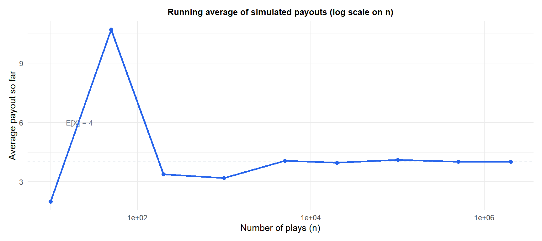
Over 2,000,000 simulated plays, the empirical average settles at 4.01 and the empirical variance at 512.45, both extremely close to the theoretical \(E[X]=4.0\) and \(\text{Var}(X)=511.5\). This is exactly the interpretation the law of large numbers gives to \(E[X]\): it is the value the sample average converges to as the number of repetitions grows, not a value any single play produces.
Expected value is not always a possible outcome
The word “expected” invites a common misreading. \(E[X]\) is a theoretical, population-level quantity, and there is no requirement that \(X\) can ever actually equal it.
⚠️ A fair die never shows 3.5
The expected value of a single fair six-sided die roll is \(E[X] = (1+2+3+4+5+6)/6 = 3.5\), a value the die physically cannot land on. “Expected” here means the long-run average over many rolls, not a prediction of what any one roll will show. The same logic applies to the payout example above: no single play of that game ever pays out exactly 4, only the average over many plays approaches it.
Running it in R
Both quantities follow directly from the probability vector, no special function needed:
x <- c(-5, 0, 10, 100)
p <- c(0.5, 0.3, 0.15, 0.05)

EX  <- sum(x * p)                  # expected value
EX2 <- sum(x^2 * p)                # E[X^2]
VarX <- EX2 - EX^2                 # variance, shortcut formula
SDX  <- sqrt(VarX)                 # standard deviation

EX; VarX; SDX

# Direct definition, should match VarX above
sum((x - EX)^2 * p)

# Simulation check: empirical mean/variance converge to EX and VarX
samples <- sample(x, size = 2e6, replace = TRUE, prob = p)
mean(samples)
var(samples)
💡 Expected value and variance of common distributions
You rarely need to compute these from scratch for a named distribution, each has a known closed form: Binomial\((n,p)\) has \(E[X]=np\) and \(\text{Var}(X)=np(1-p)\); Poisson\((\lambda)\) has \(E[X]=\text{Var}(X)=\lambda\) (the mean equals the variance, a distinctive signature of the Poisson); for a continuous Uniform\((a,b)\), \(E[X]=(a+b)/2\) and \(\text{Var}(X)=(b-a)^2/12\). The general formulas on this page are what those shortcuts are derived from.

