Law of Large Numbers

The Law of Large Numbers (LLN) is the formal guarantee behind an intuition everyone already has: flip a coin a few times and you might get an unusual run, flip it a million times and the fraction of heads will be extremely close to 50%. It is the closest relative of the Central Limit Theorem on this site, but it answers a different question, this post makes the distinction precise.

The weak law of large numbers

For independent and identically distributed random variables \(X_1, X_2, \ldots\) with finite mean \(\mu\), the sample mean \(\bar{X}_n\) converges in probability to \(\mu\):

Formally, for any \(\varepsilon > 0\): \(P(|\bar{X}_n - \mu| > \varepsilon) \to 0\) as \(n \to \infty\). In plain language: however small a margin \(\varepsilon\) you pick, the probability that the sample mean is off from the true mean by more than that margin shrinks toward zero as the sample grows.

Weak law vs strong law

The weak law above says the probability of a large deviation vanishes as \(n\) grows, but in principle it still allows the sequence \(\bar{X}_n\) to occasionally wander far from \(\mu\) infinitely often, just with vanishing probability at each fixed \(n\).

The strong law is a tighter guarantee:

\[\bar{X}_n \to \mu \quad \text{almost surely}\]

Meaning that with probability 1, the actual sequence of sample means converges to \(\mu\) and eventually stays arbitrarily close forever, not just “probably close at each \(n\)”. For nearly every practical purpose on this site, the distinction doesn’t change how you’d use the result, but it is a real and famous mathematical distinction worth knowing exists.

Worked example: the running average of die rolls

A single die is the cleanest possible case: the true mean is known exactly, so any wobble or convergence in the running average is easy to see.

Running average of die rolls converging to 3.5

Roll a single fair six-sided die repeatedly. The true mean is \(\mu = 3.5\). Track the running average as the number of rolls grows:

set.seed(7)
for (n in c(10, 100, 1000, 10000, 100000)) {
  rolls <- sample(1:6, n, replace = TRUE)
  # mean(rolls), abs(mean(rolls) - 3.5)
}

Number of rolls \(n\)	Sample mean \(\bar{X}_n\)	\(\lvert \bar{X}_n - 3.5 \rvert\)
10	3.30	0.20
100	3.43	0.07
1,000	3.538	0.038
10,000	3.5049	0.0049
100,000	3.4979	0.0021

The gap shrinks overall, but not smoothly at every step: the deviation at \(n=1{,}000\) (0.038) is still smaller than at \(n=100\) (0.07), yet in general this kind of comparison can go either way at intermediate steps. The LLN never promises that each additional roll makes the average strictly closer to \(\mu\), only that the probability of being far from \(\mu\) shrinks reliably as \(n\) grows without bound. That is exactly what “converges in probability” means: a guarantee about the long run, not a promise of smooth, step-by-step improvement.

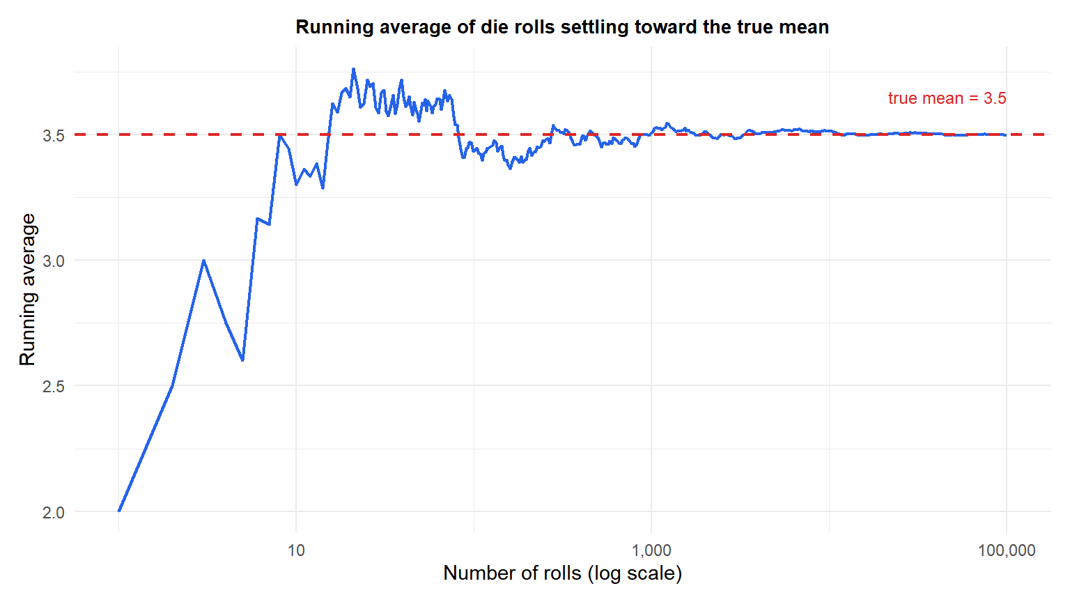
Early on, with only a handful of rolls, the running average swings widely. As the number of rolls grows into the thousands and beyond, the swings shrink and the line settles in tightly around the true mean of 3.5.

Law of Large Numbers vs Central Limit Theorem: the key difference

Both describe the behavior of \(\bar{X}_n\) as \(n\) grows, but they answer different questions.

• The LLN says WHERE \(\bar{X}_n\) ends up: it converges to the single point \(\mu\), collapsing to a point mass in the limit.
• The CLT says HOW \(\bar{X}_n\) fluctuates AROUND \(\mu\) for large but finite \(n\): approximately normally distributed, with spread shrinking as \(\sigma/\sqrt{n}\).

Put sharply: the LLN is a statement about convergence to a point; the CLT is a refinement describing the shape and rate of that convergence. If you rescale \(\bar{X}_n - \mu\) by \(\sqrt{n}\), the LLN’s “collapse to a point” becomes exactly the CLT’s normal distribution, they are two views of the same underlying convergence at different zoom levels.

Requirements for the Law of Large Numbers to hold

The observations must have a finite mean. For distributions with undefined or infinite mean, the sample mean does not converge to anything as \(n\) grows, it keeps jumping around unpredictably no matter how large the sample gets. This is a genuine, if unusual, exception worth knowing exists, most real-world quantities, with a finite mean, are safely covered by the LLN.

Running the simulation in R

The die-rolling simulation above comes from tracking a single cumulative average as the sample size climbs into the tens of thousands:

set.seed(7)
n_max <- 100000
rolls <- sample(1:6, n_max, replace = TRUE)
running_mean <- cumsum(rolls) / seq_along(rolls)

# Value at a few checkpoints
running_mean[c(10, 100, 1000, 10000, 100000)]