Cointegration and VECM
Two individually non-stationary series can still move together in a stable, predictable way over the long run, sharing what is called a common stochastic trend. When that happens they are cointegrated, and modeling them separately, or fitting a plain VAR on their raw levels, throws away real information about that long-run relationship, or worse, produces a spurious regression. This post covers how to test for cointegration and how to model it properly with a Vector Error Correction Model (VECM).
Before any of this applies, both series must first be shown to have a unit root individually, see the Dickey-Fuller test and the general stationarity post for that first step.
What cointegration means
If \(x_t\) and \(y_t\) are both \(I(1)\) (integrated of order 1: non-stationary, but stationary after one difference), they are cointegrated if some linear combination of them is itself stationary, \(I(0)\). Intuitively: both series can wander unboundedly on their own, like two separate random walks, but a specific linear combination of them stays anchored and never drifts too far from zero, because they share the same underlying stochastic trend.
\[x_t, y_t \sim I(1), \qquad y_t - \beta x_t \sim I(0)\]
\(\beta\) is the cointegrating coefficient, and \(y_t - \beta x_t\) (or more generally, including a constant, \(y_t - \beta x_t - \alpha\)) is the cointegrating relationship, interpretable as the long-run equilibrium the two series are anchored to. Classic real-world examples: spot and futures prices of the same commodity, consumption and income, exchange rates linked by purchasing power parity.
The Engle-Granger two-step method
The simplest way to test for and estimate cointegration between exactly two series.
Step 1: regress \(y_t\) on \(x_t\) by OLS and keep the residuals:
\[\hat u_t = y_t - \hat\alpha - \hat\beta x_t\]
Step 2: test whether the residuals \(\hat u_t\) are stationary using an ADF-style test. If they are, \(x_t\) and \(y_t\) are cointegrated, the OLS relationship IS the cointegrating relationship. If the residuals still have a unit root, there is no evidence of cointegration.
⚠️ Engle-Granger step 2 needs its own critical values, not the standard ADF table
The residuals \(\hat u_t\) come from an ESTIMATED regression, OLS already chose \(\hat\alpha, \hat\beta\) to fit the data as well as possible, so testing them for a unit root with the ordinary Dickey-Fuller critical values is too lenient: it will find “stationarity” (reject the unit root) too often, purely due to this estimation effect. Engle and Granger derived separate, stricter critical values (later refined further by MacKinnon) specifically for testing residuals from a cointegrating regression. Functions built for this purpose, like tseries::po.test(), apply the correct critical values automatically. A generic adf.test() on the residuals technically uses the wrong reference distribution, even though a strongly negative test statistic, as in the worked example below, will usually still clear even the stricter threshold.
Worked example: two series sharing a common trend
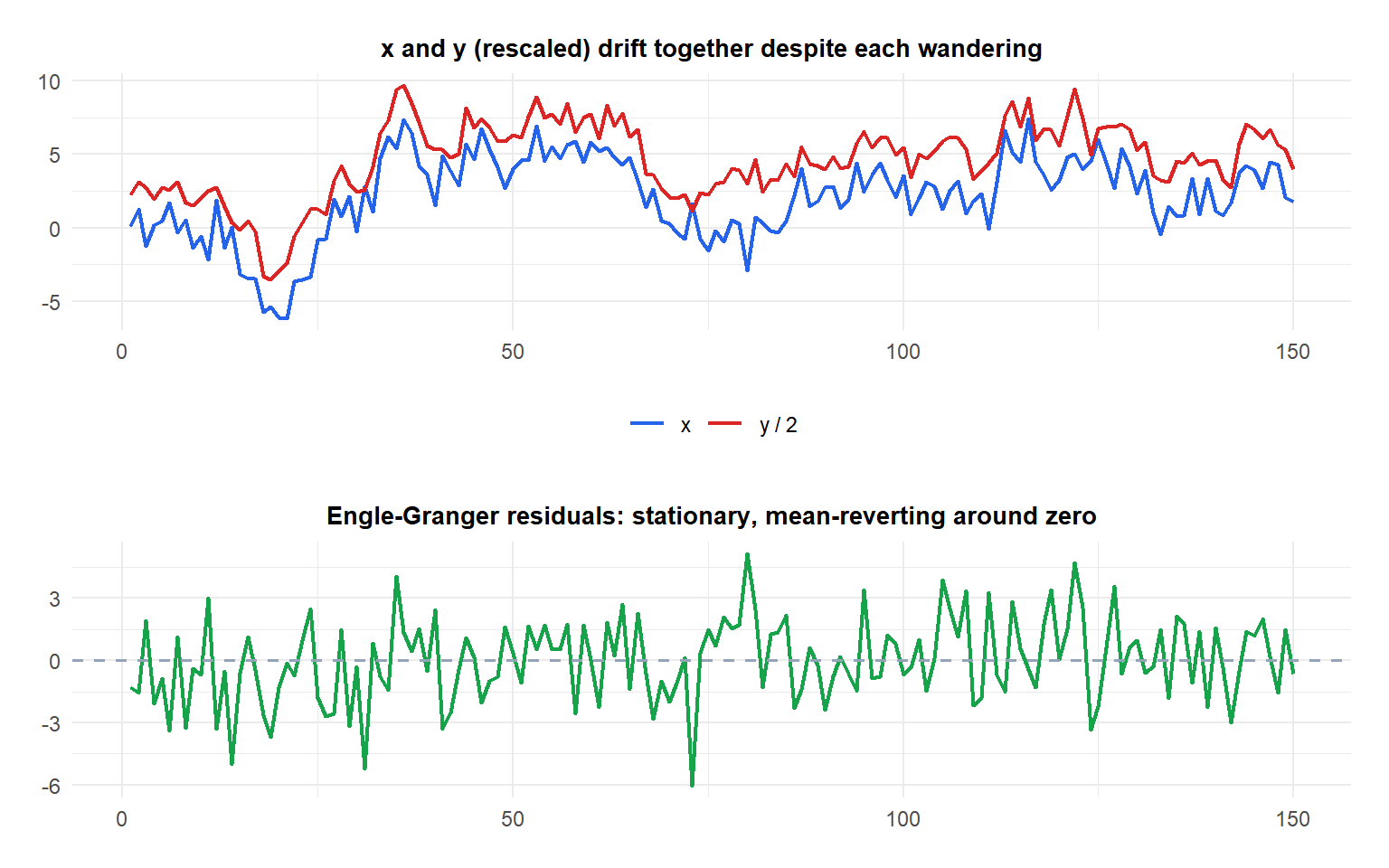
Simulating two series built from the same underlying random walk makes it possible to check, step by step, that the Engle-Granger procedure correctly recovers the cointegration that was deliberately built in.
Simulate two series that share a single common random-walk trend, so they are cointegrated by construction:
set.seed(5)
T <- 150
common_trend <- cumsum(rnorm(T))
x <- common_trend + rnorm(T, 0, 1)
y <- 2*common_trend + 5 + rnorm(T, 0, 1)
Individually, both series are non-stationary. ADF test on \(x\): test statistic \(-2.45\), \(p = 0.389\), fail to reject the unit root. ADF test on \(y\): test statistic \(-2.26\), \(p = 0.467\), fail to reject the unit root. Neither series is stationary on its own.
Engle-Granger step 1: OLS regression of \(y\) on \(x\):
\[\hat y_t = 5.659 + 1.679\, x_t\]
Both coefficients are highly significant (\(p < 0.001\)), \(R^2 = 0.845\).
Engle-Granger step 2: ADF test on the regression residuals \(\hat u_t\), using the no-constant, 1-lag specification (urca::ur.df(resid, type = "none", lags = 1)): test statistic \(= -8.286\). This is far more negative than even the strict 1% critical value for this specification (\(-2.58\)), so the unit root in the residuals is decisively rejected.
Conclusion: \(x\) and \(y\) are cointegrated, exactly as built into the simulation, since both series share the single common trend.

The Johansen test: a second, independent check
The Engle-Granger method only handles exactly 2 series and treats one as “dependent” arbitrarily. The Johansen test is more general: it works for any number of series simultaneously and does not require picking a dependent variable, based on the eigenvalues of a matrix derived from a VAR in levels. It tests, in sequence, how many cointegrating relationships exist (the cointegrating rank \(r\)): \(H_0: r = 0\) (no cointegration) vs \(r \geq 1\), then \(H_0: r \leq 1\) vs \(r \geq 2\), and so on.
Johansen trace test (urca::ca.jo(cbind(x, y), type = "trace", ecdet = "const", K = 2)) on the same simulated \(x, y\):
| Hypothesis | Test statistic | 5% critical value | Conclusion |
|---|---|---|---|
| \(r = 0\) | 72.92 | 19.96 | Reject: at least 1 cointegrating relation |
| \(r \leq 1\) | 5.92 | 7.52 | Fail to reject: no more than 1 |
Reading the table top to bottom, stop at the first row where \(H_0\) is NOT rejected, here that is \(r \leq 1\), so the cointegrating rank is \(r = 1\): exactly one cointegrating relationship, agreeing with the Engle-Granger result above and with the true simulation design, two series sharing a single common trend.
The Vector Error Correction Model (VECM)
Once cointegration is established, the right model is a VECM rather than a VAR in levels or a VAR in differences, both of which throw away information: one ignores the unit roots, the other ignores the long-run relationship. A VECM combines short-run dynamics, in differences, with an error-correction term that pulls the system back toward the long-run equilibrium whenever it drifts away.
\[\Delta \mathbf{y}_t = \boldsymbol{\alpha}(\boldsymbol{\beta}' \mathbf{y}_{t-1} - \mu) + \boldsymbol{\Gamma}_1 \Delta \mathbf{y}_{t-1} + \boldsymbol{\varepsilon}_t\]
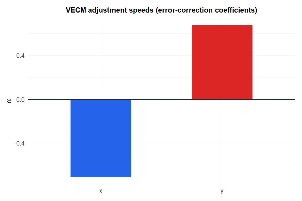
where \(\boldsymbol{\beta}' \mathbf{y}_{t-1}\) is the cointegrating relationship (how far the system was from equilibrium last period) and \(\boldsymbol{\alpha}\) is the vector of adjustment speeds, how strongly each variable corrects back toward equilibrium after a deviation.
Fitting the VECM via vars::cajorls() on the same data, at rank \(r = 1\), gives estimated adjustment speeds \(\alpha_x = -0.709\) and \(\alpha_y = +0.675\). Interpret concretely: whenever the cointegrating relationship is above its long-run equilibrium value, a positive deviation, \(x\) moves DOWN (negative coefficient) and \(y\) moves UP (positive coefficient) in the next period, both actions pushing the system back toward equilibrium, exactly the error correction the model is named for.
⚠️ Fitting a VAR in levels on cointegrated series is not just suboptimal, results can be spurious
If two non-stationary series are cointegrated and you fit a plain VAR on their raw levels, ignoring the unit roots entirely, the model is misspecified: standard errors, significance tests, and impulse responses from that VAR are not reliable. Differencing both series to force stationarity and fitting a VAR on the differences is also wrong, in a different way, it discards the long-run cointegrating relationship entirely, throwing away real information. A VECM is the specification that correctly uses both pieces: short-run dynamics from the differenced data, plus the long-run equilibrium from the level relationship.
Running it in R
The same three checks used above, the Engle-Granger residual test, the Johansen procedure, and fitting the VECM itself, each map to a single R call:
library(urca)

# Engle-Granger two-step (manual)
fit_ols <- lm(y ~ x)
resid_eg <- residuals(fit_ols)
ur.df(resid_eg, type = "none", lags = 1)   # test residuals for a unit root

# Or the built-in Engle-Granger test with correct critical values
library(tseries)
po.test(cbind(y, x))

# Johansen test
jo_test <- ca.jo(cbind(x, y), type = "trace", ecdet = "const", K = 2)
summary(jo_test)

# Fit the VECM at the chosen rank
library(vars)
vecm_fit <- cajorls(jo_test, r = 1)
summary(vecm_fit$rlm)

# Convert to a VAR in levels for forecasting, if needed
var_form <- vec2var(jo_test, r = 1)
predict(var_form, n.ahead = 12)
💡 The cointegration workflow, step by step
- Test each series individually for a unit root (Dickey-Fuller test), confirm both are \(I(1)\).
- Test for cointegration: Engle-Granger for 2 series, Johansen for 2 or more.
- If cointegrated, fit a VECM at the cointegrating rank found.
- If NOT cointegrated, either difference both series and fit a plain VAR on the differences, or reconsider whether the two series should be modeled together at all.
Skipping straight to a VAR in levels without checking any of this is the single most common mistake in applied multivariate time series work.

