Tukey's HSD test

After a significant ANOVA F-test, all you know is that at least one group mean differs from the others, not which ones. Tukey’s HSD (Honestly Significant Difference) test answers that question, testing every pairwise comparison of group means while controlling the overall (familywise) Type I error rate at the chosen \(\alpha\). ANOVA’s global F-test is a prerequisite: Tukey’s HSD is only meaningful once that test has already rejected \(H_0\).

Why not just run pairwise t-tests?

The multiple comparisons problem was already introduced in the ANOVA post, but it is worth seeing the exact numbers for this example. With \(k=3\) groups there are \(\binom{3}{2}=3\) possible pairwise comparisons. If each one is tested with a separate t-test at \(\alpha=0.05\), the probability of at least one false positive across all 3 comparisons is:

\[1 - 0.95^3 \approx 0.143\]

That is nearly three times the nominal 5% rate, just from running three tests on the same data. In general, for \(m\) independent comparisons each run at level \(\alpha\), the familywise error rate is \(1-(1-\alpha)^m\), which grows quickly: with 5 groups there are \(\binom{5}{2}=10\) comparisons and the familywise error rate climbs above 40%. Tukey’s HSD fixes this by using a wider, purpose-built critical value, so the probability of any false positive across all comparisons stays at \(\alpha\), no matter how many pairs are tested.

The studentized range distribution and the HSD formula

Tukey’s method relies on the studentized range statistic \(q\), the distribution of (largest group mean minus smallest group mean) divided by the standard error, across \(k\) independent normal groups. Instead of comparing each pair against the usual t critical value, every comparison is judged against the critical value of this range distribution, which already accounts for the fact that \(k\) means are being compared simultaneously.

For equal group sizes \(n\), the minimum difference between two means needed to be called “significant” is:

where \(q_{\alpha,k,N-k}\) is the critical value of the studentized range distribution (\(k\) = number of groups, \(N-k\) = residual/within degrees of freedom from the ANOVA), and \(MS_W\) is the within-group mean square from the ANOVA table, the same pooled variance estimate the F-test itself uses. Any pair of group means whose absolute difference exceeds HSD is declared significantly different.

The studentized range critical value \(q_{\alpha,k,N-k}\) is always larger than the corresponding two-sample t critical value would be, and it grows with \(k\): comparing more groups makes it harder for any single pair to clear the bar, which is exactly the “penalty” that keeps the familywise error rate at \(\alpha\) instead of letting it inflate with every extra comparison. When \(k=2\), there is only one possible comparison and the studentized range test reduces to an ordinary two-sample t-test.

Applying Tukey’s HSD to the diet example

The ANOVA already said the three diets are not all equal; Tukey’s HSD is what pins down exactly which pairs drive that result:

Which diets actually differ? (reusing the ANOVA example)

Recall the three-diet weight loss example: Diet A (\(n=5\), \(\bar y_A = 5.4\)), Diet B (\(n=5\), \(\bar y_B = 8.4\)), Diet C (\(n=5\), \(\bar y_C = 2.8\)). The ANOVA table gave \(MS_W = 1.100\) with \(df_W = N-k = 12\), and the overall F-test was already significant (\(F=35.70\), \(p<0.001\)), so a post-hoc comparison is justified.

The critical value of the studentized range distribution for \(k=3\) groups and \(df_W=12\) at \(\alpha=0.05\) is \(q_{0.05,3,12} = 3.773\).

\[\text{HSD} = 3.773 \times \sqrt{\frac{1.100}{5}} = 3.773 \times 0.4690 = 1.770\]

Any pairwise difference in absolute value greater than 1.770 kg is statistically significant at \(\alpha=0.05\).

Comparison	Difference	95% CI	Significant?
B \(-\) A	3.0	(1.230, 4.770)	Yes (\(p=0.0019\))
C \(-\) A	\(-2.6\)	(\(-4.370\), \(-0.830\))	Yes (\(p=0.0053\))
C \(-\) B	\(-5.6\)	(\(-7.370\), \(-3.830\))	Yes (\(p<0.0001\))

All three pairwise differences exceed 1.770 kg in absolute value, so all three are significant: Diet B produces significantly more weight loss than Diet A, which in turn produces significantly more than Diet C. The three diets form a strict ordering, not just “at least one differs”.

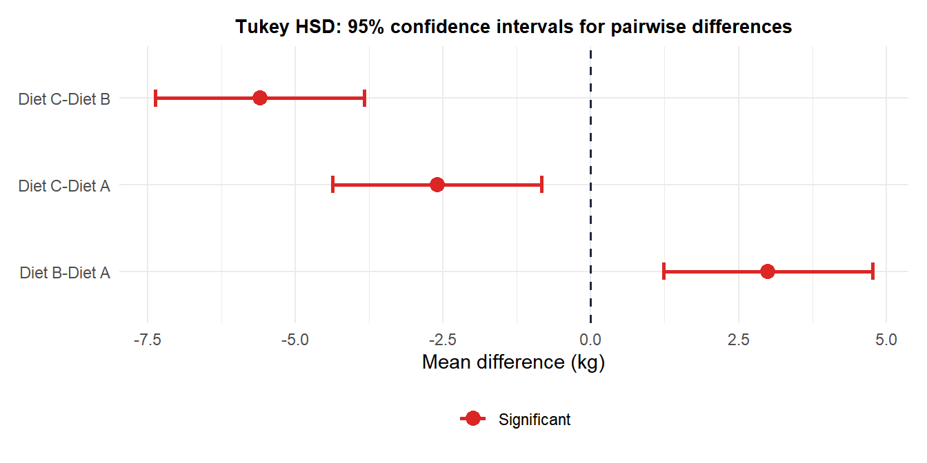
Both markers are drawn in red because every interval lies entirely to one side of 0: none of the three comparisons come close to the dashed reference line, which is consistent with three diets that are all clearly separated in effect, not just barely distinguishable at the \(\alpha=0.05\) threshold.

Reading the confidence interval directly

A pairwise confidence interval that excludes 0 is exactly equivalent to that pair being significant. For B \(-\) A, the interval (1.230, 4.770) excludes 0, which confirms significance without even needing to look at the p-value. The interval additionally tells you the plausible range for the actual size of the effect: Diet B beats Diet A by somewhere between about 1.2 and 4.8 kg, information the p-value alone never reveals. The same logic applies to the other two comparisons: neither interval contains 0, so both are significant, and both give a concrete range for the size of the difference.

Assumptions

Since Tukey’s HSD reuses the ANOVA model’s pooled variance estimate \(MS_W\), it inherits all of ANOVA’s assumptions:

• Independence: observations are independent within and across groups.
• Normality: residuals are approximately normal within each group, checked with Shapiro-Wilk or Q-Q plots.
• Homoscedasticity: equal variances across groups, checked with Levene’s test. This one matters the most for Tukey’s HSD specifically, since every single comparison uses the same pooled \(MS_W\) as its variance estimate. If one group is genuinely more variable than the others, comparisons involving that group get an estimate of spread that is too small or too large, distorting the width of every HSD interval that touches it.

Unequal group sizes are handled by a variant, the Tukey-Kramer method, which replaces \(\sqrt{MS_W/n}\) with:

\[\sqrt{\frac{MS_W}{2}\left(\frac{1}{n_i}+\frac{1}{n_j}\right)}\]

for each specific pair \(i,j\), so pairs involving smaller groups automatically get a wider, more conservative interval.

Running the test in R

TukeyHSD() takes a fitted aov() object directly and returns every pairwise comparison with its adjusted confidence interval and p-value:

loss <- c(4,5,6,5,7, 8,7,9,10,8, 3,2,4,3,2)
diet <- factor(rep(c("A","B","C"), each = 5))

fit <- aov(loss ~ diet)
summary(fit)          # confirm the omnibus F-test is significant first
TukeyHSD(fit)          # pairwise comparisons with 95% CIs
plot(TukeyHSD(fit))    # base R plot of the CIs

# Manual verification of the critical value
qtukey(0.95, nmeans = 3, df = 12)   # = 3.773

TukeyHSD() returns a diff, lwr and upr column for every pairwise comparison, giving the mean difference and its 95% confidence interval, plus a p adj column already adjusted for the number of comparisons, so it can be compared directly against \(\alpha\) without any further correction. plot(TukeyHSD(fit)) draws the same kind of interval plot shown above using base R graphics.