Polynomial regression
Polynomial regression fits a curved relationship between a predictor and a response by adding powers of \(x\), \(x^2\), \(x^3\), and so on, as extra predictors in the model. The fitted curve bends, but the model underneath is still estimated by ordinary least squares. This post shows why that is, how to spot overfitting and extrapolation problems, and how the powers of \(x\) create their own version of multicollinearity.
Still a linear model
The polynomial regression model of degree \(d\):
\[y_i = \beta_0 + \beta_1 x_i + \beta_2 x_i^2 + \dots + \beta_d x_i^d + \varepsilon_i\]
The critical point, covered in more depth in nonlinear regression, is that a model is linear or nonlinear based on whether it is linear in the parameters \(\beta_j\), not on whether the fitted curve is a straight line. Here, \(x^2\) and \(x^3\) are just additional columns of predictors: the model is still \(y = \mathbf{X}\boldsymbol{\beta} + \varepsilon\) with a bigger \(\mathbf{X}\), so ordinary least squares applies directly and there is a closed-form solution, unlike genuinely nonlinear models such as \(y = \beta_0 e^{\beta_1 x}\), which need an iterative algorithm.
Worked example: fertilizer and crop yield
Fitting a straight line, a quadratic, and a needlessly high degree to the same curved data shows exactly where each one breaks down.
A simulated dataset of \(n=45\) plots records fertilizer applied (kg/ha, 0 to about 20) and the resulting crop yield. The true relationship rises with fertilizer up to a point, then falls off as over-fertilization starts to hurt the crop, a well known real agronomic pattern that a straight line cannot capture.
Fitting three models to the same data:
| Degree | R-squared | Adjusted R-squared |
|---|---|---|
| 1 (straight line) | 0.166 | 0.147 |
| 2 (quadratic) | 0.833 | 0.825 |
| 9 | 0.859 | 0.823 |
The jump from degree 1 to degree 2 is real and large: an F-test comparing the two nested models gives \(F(1,42) = 168.24\), \(p < 0.001\), degree 2 fits dramatically better. But going from degree 2 to degree 9 barely moves R-squared (0.833 to 0.859) while the adjusted R-squared, which penalizes extra predictors, actually goes down slightly (0.825 to 0.823): the extra seven terms are not buying any real explanatory power, only fitting noise.
The quadratic fit itself: \(\widehat{\text{yield}} = 16.53 + 9.84 \cdot \text{fert} - 0.42 \cdot \text{fert}^2\), a curve that rises then turns down, exactly the shape the true process has.

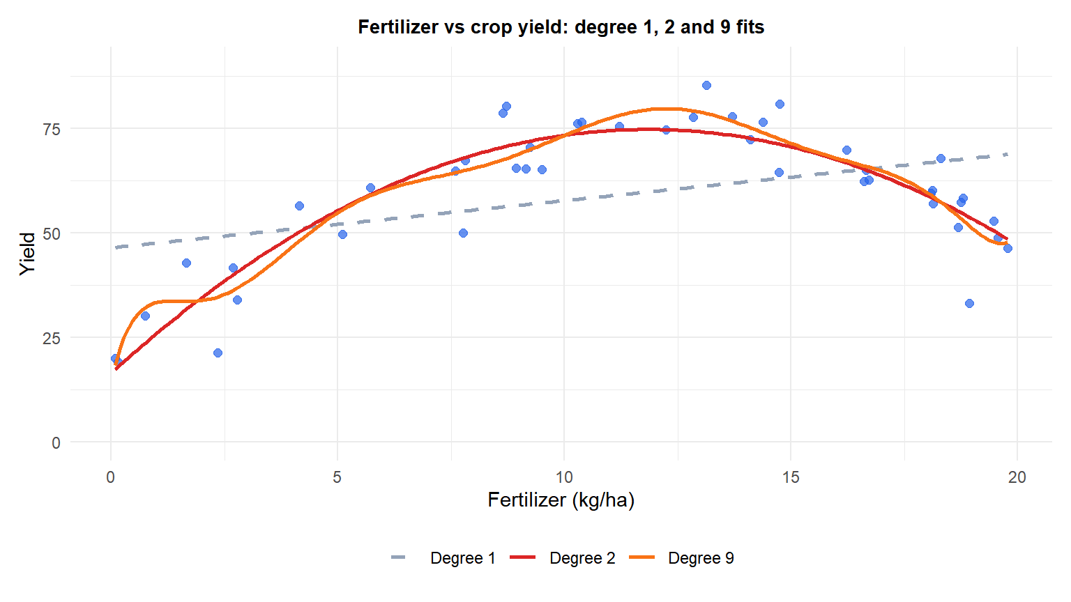
The degree 1 line (grey, dashed) cannot bend, so it underfits: it misses the early rise and the late fall entirely. The degree 2 curve (red) tracks the true rise-then-fall shape closely. The degree 9 curve (orange) wiggles between the data points, chasing noise instead of the underlying pattern, most visibly near the edges of the data.
Two real dangers: overfitting and extrapolation
The degree 9 fit above already hinted at both problems, chasing noise inside the data range and swinging wildly just outside it.
⚠️ A high degree overfits, and extrapolates worse than a straight line
Overfitting. A degree that is too high fits the noise in the sample, not the true relationship, and its adjusted R-squared can even fall even as raw R-squared keeps rising, exactly what happened above going from degree 2 to degree 9. Checking a model’s error on data it was not fit on, see cross-validation, catches this far more reliably than looking at in-sample R-squared alone.
Extrapolation. The observed fertilizer values run from about 0.1 to 19.8. Predicting just three units past the top of that range (fertilizer = 22.8), where the true curve is still a modest 27.8:
| Model | Prediction at fertilizer = 22.8 |
|---|---|
| Degree 1 | 72.1 |
| Degree 2 | 24.9 |
| Degree 9 | 820.4 |
The degree 2 model, matching the true shape, stays close to the real value. The degree 1 line, having never seen the downturn, overshoots badly. The degree 9 model explodes to a wildly implausible 820.4: high-degree polynomials curve sharply right at the edges of the training data, and that curvature swings to extreme values almost immediately outside it, a much more dangerous failure mode than a straight line ever produces.
Polynomial terms create their own multicollinearity
\(x\) and \(x^2\) are built from the same variable, so they are highly correlated by construction: here, \(\text{cor}(\text{fert}, \text{fert}^2) = 0.968\). Fitting fert + I(fert^2) directly gives both terms a VIF of 15.8, well above the common warning threshold of 5 to 10.
This does not hurt the fitted curve or its predictions, exactly as with any other multicollinearity, but it does make the individual linear and quadratic coefficients harder to interpret and less stable. Centering \(x\) first (subtracting its mean before squaring) reduces the correlation substantially; using orthogonal polynomials, which R’s poly() does by default, removes it almost entirely by construction, without changing the fitted curve at all.
Running it in R
Fitting the orthogonal and raw versions, comparing degrees, and checking VIF all take just a few lines:
💡 Fitting and comparing polynomial degrees in R
# Orthogonal polynomial (recommended, avoids the collinearity above)
fit2 <- lm(yield ~ poly(fert, 2), data = df)

# Equivalent raw polynomial (same fitted curve, correlated coefficients)
fit2_raw <- lm(yield ~ fert + I(fert^2), data = df)

# Compare nested degrees with an F-test
fit1 <- lm(yield ~ fert, data = df)
anova(fit1, fit2_raw)

# Or compare adjusted R-squared directly, see:
# /machine-learning/r-squared-adjusted-r-squared/
summary(fit1)$adj.r.squared
summary(fit2_raw)$adj.r.squared

# Multicollinearity between the polynomial terms
library(car)
vif(fit2_raw)
